LS100¶

Choosing & Running Classical Statistical Tests in Python¶

You have collected data, cleaned it, visualized it, and computed summaries. Now comes the question every research study must answer: is there any pattern, and if so, is the pattrn significant, or could it be just by chance? Classical statistical tests are the tools that answer it.

This notebook is a hands-on guide to the common tests of behavioural research: t-tests, ANOVA, correlation, regression, the chi-square test, and their non-parametric counterparts. For each of these tests, you will learn when to use it, what data structure it assumes, how to run it in Python, and how to interpret and report it honestly. We use scipy.stats and statsmodels, the two standard statistics libraries.

A theme runs through the whole notebook: a p-value is never the whole story. We will always pair it with an effect size (how big is the difference?) and think about assumptions. By the end of this notebook, you will be able to look at a research question, pick the right test, run it, and state what it does and does not show — and you will understand why, when your data has repeated measures or nesting, you need the mixed-effects models of the next notebook.

How to Use This Notebook Well¶

Run every cell yourself, top to bottom — all tests use the one dataset built in Section 0.
For each test, read the “When to use it” box first and try to decide if it fits before seeing the code.
Pay attention to the interpretation after each result. Running a test is one line; understanding it is the skill.
Mini Challenges and Checkpoints are for you. The final decision guide (Section 7) is worth bookmarking.

A word of caution up front: statistics is easy to run and easy to misuse. This notebook teaches the mechanics and the good habits — effect sizes, assumption checks, and honesty about multiple comparisons — that separate an genuine analysis from “p-hacking”.

Table of Content:¶

Section 0: Setup & Our Dataset¶

We import

NumPy and pandas for data handling,
scipy.stats (the test functions) and statsmodels (regression, ANOVA tables, post-hoc tests).
matplotlib /seaborn for creating plots — remember from Notebook 03 that it is always a good practice to visualize the data before conducting further analyses.

# If you don't have scipy statsmodels installed, uncomment the following line to install it:
# !pip install scipy
# !pip install statsmodels

import numpy as np
import pandas as pd
import matplotlib.pyplot as plt
import seaborn as sns
from scipy import stats
import statsmodels.formula.api as smf
import statsmodels.api as sm

print("scipy   :", __import__("scipy").__version__)
print("statsmodels:", sm.__version__)

scipy   : 1.16.3
statsmodels: 0.14.5

We simulate a tidy dataset from a fictional learning study. Sixty participants — half novices, half experts — each trained with one of three methods (massed, spaced, interleaved), logged their practice hours, and were scored on a task. We also recorded a score for “balance” before and after a short intervention (a paired measure), and whether each participant ultimately passed. A fixed random seed keeps the numbers reproducible.

rng = np.random.default_rng(7)
n = 60

group = np.repeat(["novice", "expert"], n // 2)          # 30 novices, 30 experts
method = rng.choice(["massed", "spaced", "interleaved"], size=n)
practice_hours = rng.uniform(0, 20, n)

# Score is built from real effects: experts score higher, methods differ,
# and more practice helps -- plus random noise. (This is the "ground truth"
# the tests below will try to recover.)
group_effect  = np.where(group == "expert", 10.0, 0.0)
method_effect = np.select([method == "massed", method == "spaced", method == "interleaved"],
                          [0.0, 4.0, 8.0])
score = (55 + group_effect + method_effect + 0.8 * practice_hours
         + rng.normal(0, 7, n)).clip(0, 100)

# Reaction time (seconds): experts are faster. Independent of score.
reaction_time = np.where(group == "expert",
                         rng.normal(0.62, 0.12, n),
                         rng.normal(0.78, 0.15, n))

# A paired measure: balance score before and after an intervention (improves ~4 points).
balance_pre = rng.normal(70, 9, n)
balance_post = balance_pre + rng.normal(4, 5, n)

# Categorical outcome for the chi-square test.
passed = np.where(score >= 75, "pass", "fail")

df = pd.DataFrame({
    "participant": np.arange(1, n + 1),
    "group": group, "method": method,
    "practice_hours": practice_hours.round(1),
    "score": score.round(1), "reaction_time": reaction_time.round(3),
    "balance_pre": balance_pre.round(1), "balance_post": balance_post.round(1),
    "passed": passed,
})
print("Shape:", df.shape)
df.head()

Shape: (60, 9)

Section 1: The Logic of Hypothesis Testing¶

Before any specific test, you need the shared logic they all run on. It is a kind of proof by contradiction.

Key Characteristics:

Null hypothesis ( $H_0$ ): the “boring” claim that there is no effect (no difference, no relationship). This is what we try to disprove.
Alternative hypothesis ( $H_1$ ): the claim that there is an effect.
p-value: the probability of seeing data at least this extreme if $H_0$ were true. A small p-value means “this data would be surprising under the null”, which is evidence against the null.
Significance level (alpha): the threshold we fix in advance, conventionally 0.05. If p < alpha we “reject $H_0$ ”.
Type I error (false positive): rejecting $H_0$ when it is actually true. Its rate is alpha.
Type II error (false negative): failing to detect a real effect.

Three warnings that prevent most misuse:

p is not the probability that $H_0$ is true, and “p > 0.05” is not proof of no effect — only a failure to find one.
Statistical significance is not importance. With enough data, a trivial difference can be “significant”. Always report an effect size.
Decide your test and alpha before looking for significance, not after.

Section 2: Descriptive Statistics & Confidence Intervals¶

Tests compare summaries, so start there. Beyond the mean and standard deviation (SD) you met in Notebook 01, two more matter for inference:

Standard error of the mean (SE): how much the sample mean would wobble if you repeated the study. It shrinks as the sample grows: SE = SD / sqrt(n).
95% confidence interval (CI): a range that would contain the true mean in 95% of repeated studies. A CI is often more informative than a p-value because it shows both the estimate and its uncertainty in the data’s own units.

# Group-wise descriptives for the task score.
print(df.groupby("group")["score"].describe()[["count", "mean", "std"]], "\n")

# 95% CI for each group's mean score, using the t-distribution.
for g, sub in df.groupby("group"):
    m = sub["score"].mean()
    sem = stats.sem(sub["score"])     # SD / sqrt(n)
    lo, hi = stats.t.interval(0.95, len(sub) - 1, loc=m, scale=sem)
    print(f"{g:7s}: mean = {m:5.1f}, 95% CI [{lo:.1f}, {hi:.1f}]")

        count       mean       std
group                             
expert   30.0  76.540000  9.737046
novice   30.0  66.003333  9.536373 

expert : mean =  76.5, 95% CI [72.9, 80.2]
novice : mean =  66.0, 95% CI [62.4, 69.6]

Mini Challenge 2. Compute the mean and 95% CI of reaction_time for each group. Do the two intervals overlap? (Overlap is a hint, not a test — Section 4 makes it rigorous.)

Section 3: Checking Assumptions¶

Most “classical” tests are parametric — they assume the data behaves a certain way. The big three assumptions are:

Normality — values are roughly bell-shaped (matters most for small samples).
Equal variance (homogeneity) — groups being compared have similar spread.
Independence — observations do not influence each other. This one is about study design, not something a test can rescue — and it is exactly what breaks with repeated measures (see Section 8).

Two quick formal checks: Shapiro–Wilk for normality and Levene’s test for equal variance. For these, the null is “assumption holds”, so a small p-value means the assumption is violated.

expert_score = df.loc[df["group"] == "expert", "score"]
novice_score = df.loc[df["group"] == "novice", "score"]

# Shapiro-Wilk: H0 = data is normal. p > 0.05 -> normality is reasonable.
for name, x in [("expert", expert_score), ("novice", novice_score)]:
    w, p = stats.shapiro(x)
    verdict = "looks normal" if p > 0.05 else "NOT normal"
    print(f"Shapiro {name}: W={w:.3f}, p={p:.3f} -> {verdict}")

# Levene: H0 = equal variances. p > 0.05 -> equal-variance assumption is reasonable.
lev_stat, lev_p = stats.levene(expert_score, novice_score)
print(f"\nLevene: stat={lev_stat:.3f}, p={lev_p:.3f} -> "
      f"{'equal variances OK' if lev_p > 0.05 else 'variances DIFFER'}")

Shapiro expert: W=0.966, p=0.446 -> looks normal
Shapiro novice: W=0.914, p=0.019 -> NOT normal

Levene: stat=0.387, p=0.536 -> equal variances OK

Good habit: also look at the data (a histogram or boxplot from Notebook 03) rather than trusting these tests alone — with small samples they have little power, and with huge samples they flag trivial deviations. When normality or equal variance clearly fails, switch to the non-parametric tests in Section 5 (or use Welch’s t-test, below, which does not assume equal variance).

Section 4: Comparing Means¶

The most common research question: do these groups differ on average? The right tool depends on how many groups and whether observations are paired.

4.1. One-Sample t-test — “does the mean differ from a fixed value?”¶

When to use it: you have one group and want to compare its mean to a known benchmark (a chance level, a published norm, a target). H0: the population mean equals that value.

# Is the average task score different from a curriculum benchmark of 70?
benchmark = 70
t_stat, p = stats.ttest_1samp(df["score"], benchmark)
print(f"Mean score = {df['score'].mean():.1f} (benchmark {benchmark})")
print(f"One-sample t-test: t = {t_stat:.2f}, p = {p:.4f}")
print("->", "differs from benchmark" if p < 0.05 else "no evidence it differs")

Mean score = 71.3 (benchmark 70)
One-sample t-test: t = 0.90, p = 0.3713
-> no evidence it differs

4.2. Independent Two-Sample t-test — “do two separate groups differ?”¶

When to use it: two independent groups (different participants), one numeric outcome. H0: the two population means are equal.

A practical note: the classic Student’s t-test assumes equal variances; Welch’s t-test does not and is the safer default. We report both, plus Cohen’s d, the standard effect size (≈ 0.2 small, 0.5 medium, 0.8 large).

def cohens_d(a, b):
    """Standardised mean difference between two independent samples."""
    a, b = np.asarray(a), np.asarray(b)
    na, nb = len(a), len(b)
    pooled_sd = np.sqrt(((na - 1) * a.std(ddof=1)**2 + (nb - 1) * b.std(ddof=1)**2)
                        / (na + nb - 2))
    return (a.mean() - b.mean()) / pooled_sd

# Do experts and novices differ in reaction time?
exp_rt = df.loc[df["group"] == "expert", "reaction_time"]
nov_rt = df.loc[df["group"] == "novice", "reaction_time"]

t_student, p_student = stats.ttest_ind(exp_rt, nov_rt, equal_var=True)   # Student
t_welch,   p_welch   = stats.ttest_ind(exp_rt, nov_rt, equal_var=False)  # Welch (safer)
d = cohens_d(exp_rt, nov_rt)

print(f"Expert mean RT = {exp_rt.mean():.3f}s | Novice mean RT = {nov_rt.mean():.3f}s")
print(f"Student t-test: t={t_student:.2f}, p={p_student:.4f}")
print(f"Welch  t-test: t={t_welch:.2f}, p={p_welch:.4f}")
print(f"Cohen's d = {d:.2f}  (effect size)")
print("->", "groups differ" if p_welch < 0.05 else "no evidence of difference")

Expert mean RT = 0.651s | Novice mean RT = 0.729s
Student t-test: t=-2.47, p=0.0167
Welch  t-test: t=-2.47, p=0.0168
Cohen's d = -0.64  (effect size)
-> groups differ

4.3. Paired t-test — “did the same subjects change?”¶

When to use it: two measurements on the same participants (before/after, condition A vs B within-subject). Because each person is their own control, this test is far more powerful than treating the two columns as independent groups. H0: the mean difference is zero.

# Did balance scores change from before to after the intervention?
t_stat, p = stats.ttest_rel(df["balance_post"], df["balance_pre"])
diff = df["balance_post"] - df["balance_pre"]
# Cohen's d for paired data: mean difference / SD of differences.
d_paired = diff.mean() / diff.std(ddof=1)

print(f"Mean change = {diff.mean():+.2f} points (SD {diff.std(ddof=1):.2f})")
print(f"Paired t-test: t = {t_stat:.2f}, p = {p:.4f}, Cohen's d = {d_paired:.2f}")
print("->", "significant change" if p < 0.05 else "no significant change")

Mean change = +4.14 points (SD 4.95)
Paired t-test: t = 6.48, p = 0.0000, Cohen's d = 0.84
-> significant change

4.4. One-Way ANOVA — “do 3 or more groups differ?”¶

When to use it: three or more groups, one numeric outcome. Why not run many t-tests? Because each test carries a 5% false-positive risk, and those risks pile up (the multiple-comparisons problem of Section 7). ANOVA asks one overall question: are these group means all equal? H0: all group means are equal.

A significant ANOVA tells you some group differs but not which. For that you run a post-hoc test — Tukey’s HSD — which compares every pair while controlling the overall error rate. We also report eta-squared, the share of variance explained (≈ 0.01 small, 0.06 medium, 0.14 large).

# Does the training METHOD affect score?
groups = [df.loc[df["method"] == m, "score"] for m in ["massed", "spaced", "interleaved"]]
f_stat, p = stats.f_oneway(*groups)
print(f"One-way ANOVA: F = {f_stat:.2f}, p = {p:.4f}")

# Eta-squared via the statsmodels ANOVA table (SS_between / SS_total).
model = smf.ols("score ~ C(method)", data=df).fit()
aov = sm.stats.anova_lm(model, typ=2)
eta_sq = aov.loc["C(method)", "sum_sq"] / aov["sum_sq"].sum()
print(f"Eta-squared = {eta_sq:.3f}")
print("->", "at least one method differs" if p < 0.05 else "no evidence methods differ")

One-way ANOVA: F = 8.22, p = 0.0007
Eta-squared = 0.224
-> at least one method differs

# Post-hoc: WHICH methods differ? Tukey HSD compares all pairs safely.
from statsmodels.stats.multicomp import pairwise_tukeyhsd
tukey = pairwise_tukeyhsd(endog=df["score"], groups=df["method"], alpha=0.05)
print(tukey)
# 'reject = True' marks pairs that differ significantly.

   Multiple Comparison of Means - Tukey HSD, FWER=0.05   
=========================================================
   group1   group2 meandiff p-adj   lower   upper  reject
---------------------------------------------------------
interleaved massed  -8.6231 0.0242   -16.3 -0.9462   True
interleaved spaced   4.4766 0.2923 -2.6409 11.5942  False
     massed spaced  13.0997 0.0005  5.2743 20.9251   True
---------------------------------------------------------

Checkpoint 4. Match the question to the test: one group vs a number → one-sample t; two independent groups → independent t (Welch); one group measured twice → paired t; three+ groups → ANOVA + Tukey. If you can do this matching from memory, you have the core of comparing means.

Section 5: When Assumptions Fail — Non-Parametric Tests¶

When normality is clearly violated, your sample is tiny, or the outcome is ordinal (ranks, Likert scales), use a non-parametric test. These work on the ranks of the data rather than the raw values, so they make no normality assumption. Each parametric test has a direct counterpart:

Parametric (Section 4)	Non-parametric counterpart
Independent t-test	Mann–Whitney U
Paired t-test	Wilcoxon signed-rank
One-way ANOVA	Kruskal–Wallis

They are slightly less powerful when the data is normal, but far more trustworthy when it is not.

# Mann-Whitney U: independent groups, no normality assumption (vs 4.2)
u_stat, p_mw = stats.mannwhitneyu(exp_rt, nov_rt, alternative="two-sided")
print(f"Mann-Whitney U: U = {u_stat:.0f}, p = {p_mw:.4f}")

# Wilcoxon signed-rank: paired data (vs 4.3)
w_stat, p_w = stats.wilcoxon(df["balance_post"], df["balance_pre"])
print(f"Wilcoxon signed-rank: W = {w_stat:.0f}, p = {p_w:.4f}")

# Kruskal-Wallis: 3+ groups (vs 4.4)
h_stat, p_kw = stats.kruskal(*groups)
print(f"Kruskal-Wallis: H = {h_stat:.2f}, p = {p_kw:.4f}")

Mann-Whitney U: U = 292, p = 0.0199
Wilcoxon signed-rank: W = 218, p = 0.0000
Kruskal-Wallis: H = 11.28, p = 0.0036

Notice these conclusions agree with the parametric tests above — reassuring, and exactly what you hope to see when assumptions are only mildly stretched. When parametric and non-parametric disagree, trust the non-parametric result and report it.

Section 6: Measuring Relationships¶

The other big family of questions: not “do groups differ?” but “do two variables move together?”

6.1. Correlation — “do two numeric variables vary together?”¶

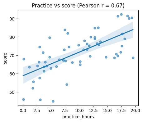
When to use it: two numeric variables, one observation per subject. The correlation coefficient r runs from -1 to +1 (0 = no linear relationship). Pearson’s r measures linear association and assumes roughly normal data; Spearman’s works on ranks and catches any monotonic relationship, so it is robust to outliers and non-linearity.

The eternal reminder: correlation is not causation. A relationship can arise from a hidden third variable.

# Do practice hours relate to score?
r_pearson, p_pearson = stats.pearsonr(df["practice_hours"], df["score"])
r_spearman, p_spearman = stats.spearmanr(df["practice_hours"], df["score"])
print(f"Pearson  r = {r_pearson:.2f}, p = {p_pearson:.4f}  (linear)")
print(f"Spearman r = {r_spearman:.2f}, p = {p_spearman:.4f}  (monotonic, robust)")

# Always plot the relationship you are correlating.
fig, ax = plt.subplots(figsize=(5, 4))
sns.regplot(data=df, x="practice_hours", y="score", ax=ax,
            scatter_kws={"alpha": 0.6, "s": 25})
ax.set_title(f"Practice vs score (Pearson r = {r_pearson:.2f})")
plt.show()

Pearson  r = 0.67, p = 0.0000  (linear)
Spearman r = 0.69, p = 0.0000  (monotonic, robust)

6.2. Simple Linear Regression — “how much does Y change per unit of X?”¶

When to use it: like correlation, but you want a predictive equation, score = intercept + slope * practice_hours. Regression gives you the slope (the change in Y for a one-unit rise in X), a significance test for it, and R² (the fraction of variance explained). We use statsmodels, whose summary table is the standard in research reporting — and the same engine behind the mixed-effects models next notebook.

# Fit score ~ practice_hours with ordinary least squares (OLS).
model = smf.ols("score ~ practice_hours", data=df).fit()
print(model.summary().tables[1])      # the coefficients table

slope = model.params["practice_hours"]
r2 = model.rsquared
print(f"\nInterpretation: each extra hour of practice predicts "
      f"{slope:+.2f} points of score.")
print(f"R-squared = {r2:.2f}  ->  practice explains {r2:.0%} of the variance in score.")

==================================================================================
                     coef    std err          t      P>|t|      [0.025      0.975]
----------------------------------------------------------------------------------
Intercept         58.7576      2.096     28.033      0.000      54.562      62.953
practice_hours     1.2863      0.186      6.908      0.000       0.914       1.659
==================================================================================

Interpretation: each extra hour of practice predicts +1.29 points of score.
R-squared = 0.45  ->  practice explains 45% of the variance in score.

6.3. Chi-Square Test — “are two categorical variables associated?”¶

When to use it: both variables are categories (group membership, pass/fail, behaviour type). It compares the counts you observed against the counts you’d expect if the two variables were unrelated. H0: the variables are independent.

# Are 'group' and 'passed' associated? Start with a contingency table of counts.
contingency = pd.crosstab(df["group"], df["passed"])
print("Observed counts:")
print(contingency, "\n")

chi2, p, dof, expected = stats.chi2_contingency(contingency)
print(f"Chi-square = {chi2:.2f}, dof = {dof}, p = {p:.4f}")
print("->", "group and outcome ARE associated" if p < 0.05
      else "no evidence of association")

Observed counts:
passed  fail  pass
group             
expert    12    18
novice    26     4 

Chi-square = 12.13, dof = 1, p = 0.0005
-> group and outcome ARE associated

Mini Challenge 6. Build a contingency table of method × passed and run a chi-square test. Are some training methods linked to higher pass rates? (Watch the small cell counts — chi-square gets unreliable when expected counts drop below ~5.)

Section 7: Choosing the Right Test & the Multiple-Comparisons Trap¶

A decision guide¶

Work down these questions:

Your question	Outcome type	Situation	Test
Mean vs a fixed value	numeric	one group	one-sample t (or Wilcoxon)
Two groups differ?	numeric	independent	independent t / Welch (or Mann–Whitney)
Same subjects changed?	numeric	paired	paired t (or Wilcoxon signed-rank)
3+ groups differ?	numeric	independent	one-way ANOVA + Tukey (or Kruskal–Wallis)
Two variables move together?	numeric	—	Pearson / Spearman correlation
Predict Y from X?	numeric	—	linear regression
Two categories associated?	categorical	—	chi-square

The non-parametric option in brackets is your fallback when normality fails or the data is ordinal.

The multiple-comparisons trap¶

Every test at alpha = 0.05 has a 5% false-positive rate. Run 20 tests on noise and, on average, one will look “significant” by chance. So:

Decide your key comparisons in advance; do not fish through every pair.
When you must run many tests, correct for it — Tukey’s HSD (Section 4.4) does this for you, and methods like Bonferroni (divide alpha by the number of tests) do it generally.

# The trap, demonstrated. Imagine many studies, each running 20 t-tests on PURE
# NOISE (no real effects). How many "significant" hits show up per study?
per_study_hits = []
for study in range(1000):
    hits = sum(stats.ttest_ind(rng.normal(0, 1, 30), rng.normal(0, 1, 30))[1] < 0.05
               for _ in range(20))
    per_study_hits.append(hits)

print(f"Average false positives per 20-test study: {np.mean(per_study_hits):.2f}")
print(f"Studies with at least one false 'hit'    : {np.mean(np.array(per_study_hits) > 0):.0%}")
print("So with 20 tests you should EXPECT ~1 significant result even when nothing is real.")
print("Bonferroni fix: with 20 tests, use alpha = 0.05/20 =", round(0.05 / 20, 4))

Average false positives per 20-test study: 0.98
Studies with at least one false 'hit'    : 62%
So with 20 tests you should EXPECT ~1 significant result even when nothing is real.
Bonferroni fix: with 20 tests, use alpha = 0.05/20 = 0.0025

Section 8: Bridge to Mixed-Effects Models + Weekly Challenge¶

Every test in this notebook rests on independence — each observation standing on its own. But behavioural data often violates this in a specific way: you measure the same subject many times (many frames per athlete, many trials per participant, many recordings per animal). Those repeated measurements are correlated — an athlete who is fast on trial 1 tends to be fast on trial 2 — and a plain t-test or ANOVA treats them as if they were independent, badly overstating your evidence.

The fix is a model that explicitly accounts for the structure: a linear mixed-effects model, which adds a “random effect” for each subject. That is exactly where the next notebook, Intro to Mixed-Effects Models, begins — with the question “why is a simple t-test not enough?” You now have the full answer: because the t-test assumes independence that repeated-measures data does not have.

Weekly Challenge. Take a research question of your own (or reuse df) and run a complete mini-analysis:
State your H0 and H1 in one sentence each.
Pick the right test using the Section 7 guide, and justify the choice.
Check the relevant assumptions (Section 3).
Run the test and report the result properly: the statistic, the p-value, an effect size, and a 95% CI or group means.
Write a one-sentence plain-language conclusion — and one sentence on what the test does not prove.
Doing all five, every time, is what turns “running statistics” into “doing statistics”.

End of Notebook. Next in this module: Intro to Linear Mixed-Effects Models, for when your data has repeated measures or nesting that these classical tests cannot handle.