Last updated: 2026-07-28
Authored by Souvik Mandal, Ph.D.
Project Leader & Instructor, Computational Behavioral Sciences, LS100, FAS, Harvard University | Linkedin ID: souvik-mandal-phd
Table of Contents
Introduction: Turning the Visible World into Data
Who does not capture time, joy, and memories through recording videos with our smartphones? It feels ordinary, but the path to freezing time in a visual media rests on a remarkable history. Early photography in 1839 made it possible to preserve a single moment. Motion studies in the 1870s showed that movement could be broken into analyzable visual stages, and cinema in the 1890s made continuous motion replayable. When digital cameras became widely accessible in laboratories, classrooms, and consumer devices during the 1990s and 2000s, recorded motion entered another era. While films were primarily used to preserved and replayed motion, digital video does something quite extraordinary - it stores scenes as data - pixels arranged into frames and indexed in time, allowing light, color, shape, and motion to be measured, processed, and analyzed computationally. That shift is one reason digital cameras became integral to scientific studies across the behavioral, biological, medical, and social sciences.
This guide introduces the foundational ideas behind that transformation. How does a camera convert light into digital values? What is a pixel, and why do resolution and bit depth matter? How do frame rate, shutter speed, and sensor design affect what can be measured? By understanding these ideas, we can begin to see digital video not just as media, but as a scientific tool that represents the visual world.
Optics, Exposure, and the Measurement Tradeoffs
If digital video turns the visible world into data, optics determine what version of that world reaches the image sensor in the first place. Anyone who has tried to record a fast-moving pet indoors, a dimly lit concert, or a bright sunset has seen this directly: the same moment can appear sharp or blurry, bright or noisy, wide or tightly framed depending on how the camera is set. These differences are not only aesthetic. They determine what visual information is available to be recorded at all.
Before light hits the sensor and any pixel values are stored, light first passes through the camera lens. The optics shape how much light enters the camera, how much of the scene is included, and which parts of the scene appear in sharp focus. Four ideas are especially important for digital video literacy:
Aperture: The opening in the lens that controls how much light enters the camera. A wider aperture admits more light, which helps in dim conditions, but it also reduces depth of field, leaving only a certain distance of the scene sharply focused.
Shutter speed: The duration for which the sensor is exposed to light for each frame. Faster shutter speeds reduce motion blur and make rapid actions easier to inspect, but they also collect less light.
ISO: The amplification applied to the recorded signal. Increasing ISO can brighten a dark scene, but it also amplifies noise and can obscure subtle visual details.
Focal length: A property of the lens that influences field of view and apparent magnification. Shorter focal lengths capture more of a scene, which can be useful for large arenas or group settings, whereas longer focal lengths narrow the view and make distant subjects appear larger.
Aperture, shutter speed, and ISO are often described as the exposure triangle because they jointly determine how bright, sharp, and noisy a frame will be. In practice, however, they are best understood as tradeoffs rather than independent settings. A fast shutter may be ideal for inspecting wing beats, hand gestures, or eye movements, but it also shortens the time available to collect light. To compensate, one may need a wider aperture, a higher ISO, stronger illumination, or eventually a sensor that performs better in low light.
This is why optics and sensor choice cannot be separated. A camera is not simply collecting a scene; it is selecting what aspects of that scene can be captured clearly enough to matter later. If a study requires high frame rates in dim conditions, the central question is not which camera looks best, but which optical and sensor combination preserves the information the study depends on. In that sense, camera setup is part of the measurement design itself.
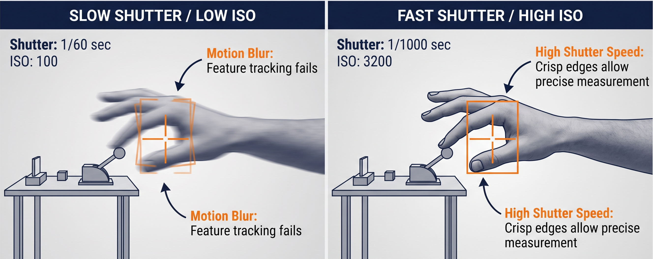
Figure 01: Optics and exposure tradeoffs in digital video. Aperture, shutter speed, ISO, and focal length shape how much light is recorded, how motion appears, how much of the scene is visible, and how much noise enters the final image.
Pixels, Color, and the Digital Image
Once light has passed through the optics and reached the sensor, the camera still has one more transformation to perform: it must convert a visual scene into a form that a computer can store. That form is the digital image, a grid of pixels in which each pixel holds numerical information about a tiny portion of the scene. If a frame is 1920 by 1080 pixels, then it contains 2,073,600 pixel locations, each acting as a small measurement site.
To the eye, a scene feels visually continuous. To a computer, that same scene becomes an organized array of numbers. In grayscale imaging, each pixel stores a single intensity value. In color imaging, each pixel usually stores three values corresponding to red, green, and blue. That is why a grayscale image can be represented in Python as a two-dimensional NumPy array with shape , while a color image can be represented as a three-dimensional array with shape . When frames are arranged over time, video extends this same logic one step further.
This array-based view matters because it turns images into data that can be indexed, compared, sliced, and measured. Bright regions, edges, shadows, textures, and color differences do not exist only as visual impressions. They also exist as patterns in structured numerical values.
Bit depth determines how precisely those values can be recorded. The basic rule is simple: if a channel uses bits, it can store possible values. It helps to start with grayscale examples:
1-bit: A pixel can store only values, such as 0 for dark and 1 for bright.
2-bit: A pixel can store values, such as 00, 01, 10, and 11, which can represent absolute dark, dark gray, light gray, and absolute bright.
As bit depth increases, the steps between brightness levels become finer. If a single channel uses 8 bits, it can represent possible intensity levels. In a standard RGB image, each pixel combines one red, one green, and one blue value. The total number of possible color combinations is therefore:
That is why people often say an 8-bit RGB image can display about 16.8 million colors. If the bit depth rises to 10 bits per channel, each channel can represent levels, and the total number of possible colors becomes:
Higher bit depth does not simply increase a headline number of colors. It allows finer gradations of brightness and color, which can matter when shadows, subtle contrasts, or low-light details carry useful information. To a casual viewer, these differences may seem minor. For measurement and analysis, they can be substantial.
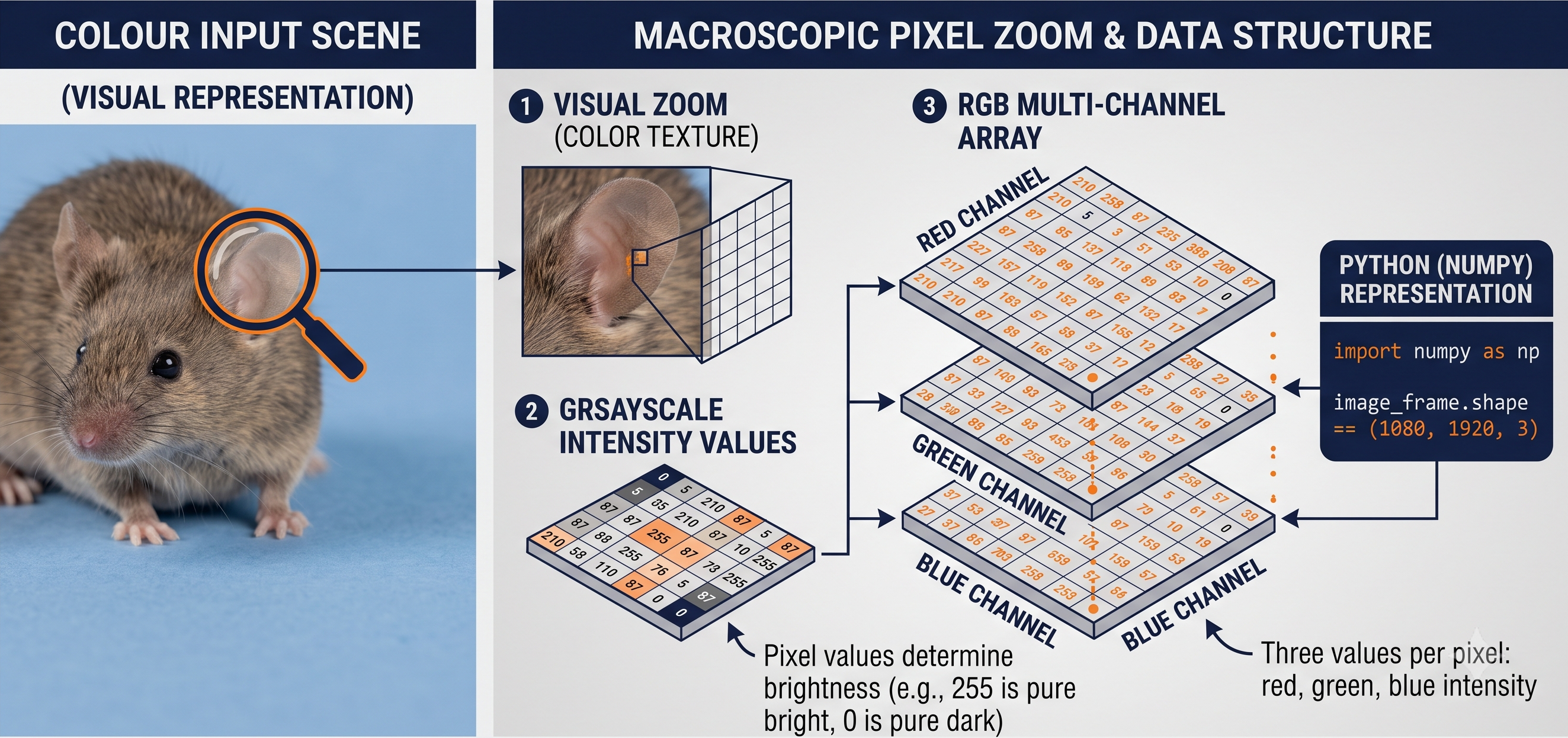
Figure 02: A digital image as a pixel grid and a multi-channel array. Each pixel stores numerical measurements, and bit depth determines how finely brightness and color can be represented.
Sensors: Where Light Becomes Measurement
If pixels are the numerical units a computer reads, the sensor is the physical surface that makes those numbers possible. Beneath the lens sits an array of light-sensitive sites, often called photosites, that collect incoming photons during each exposure and convert them into electrical signals. Those signals are then processed into the pixel values that appear in a digital image or video frame. In that sense, the sensor is where the visible world stops being only light and begins to become measurement.
Not all sensors perform that task in the same way. Two cameras may both record 1920 by 1080 video, yet differ substantially in brightness, noise, field of view, color fidelity, or performance at high frame rates. The reason is that a sensor is not defined only by how many pixels it produces. Its physical size, internal architecture, and readout design all influence what kind of data the camera can record.
One important property is sensor size. Categories such as smartphone sensors, Micro Four Thirds, APS-C, and full frame refer to the physical dimensions of the light-sensitive surface. Larger sensors can often collect more total light, especially when paired with larger photosites, which can improve low-light performance and reduce noise. Sensor size also interacts with lens choice, affecting field of view and depth of field. This is why two cameras with the same resolution can still produce very different images.
Another important property is the relationship between pixel count and photosite size. A sensor with more pixels can record finer spatial detail, but if those pixels are packed tightly onto a very small sensor, each photosite may collect less light. That can make noise more visible and can make high-frame-rate recording harder in dim conditions. More megapixels do not automatically mean better measurement. In many settings, the more important question is whether the sensor can capture the relevant detail clearly enough under the lighting and speed constraints of the study.
Sensors also differ in whether they are designed primarily for color or monochrome imaging. Most everyday cameras use color sensors with a filter array, often based on red, green, and blue elements, so that color can be reconstructed from the incoming light. Monochrome sensors do not divide incoming light into color channels in the same way, which can make them more light-sensitive. If a study depends mainly on contrast, motion, or timing rather than color information, a monochrome sensor may sometimes be a better measurement tool.
The two sensor architectures students will encounter most often are CCD and CMOS. CCD sensors were historically important in digital imaging and are known for strong image uniformity in some applications. CMOS sensors, however, dominate modern cameras because they are faster to read out, consume less power, and are easier to integrate with the rest of the camera electronics. That makes CMOS especially important for smartphones, high-frame-rate video, and most modern scientific and consumer cameras.
Finally, it is useful to distinguish between rolling shutter and global shutter behavior. Many CMOS sensors read the frame line by line rather than all at once. This rolling readout can distort very fast motion or rapid camera movement, causing slanted or skewed shapes. A global shutter records the entire frame simultaneously, which is often preferable when precise motion timing matters. For behavioral research, this difference can be important when the goal is not simply to view motion, but to measure it accurately.
Taken together, these features explain why sensor choice is never just a matter of brand or image quality. It is a decision about what kind of visual evidence can be captured reliably. A larger APS-C sensor may be helpful for low-light recording, a monochrome sensor may be better for contrast-based tracking, and a global-shutter camera may be essential for very fast movement. The best sensor is not the most expensive one. It is the one that preserves the information the study needs.
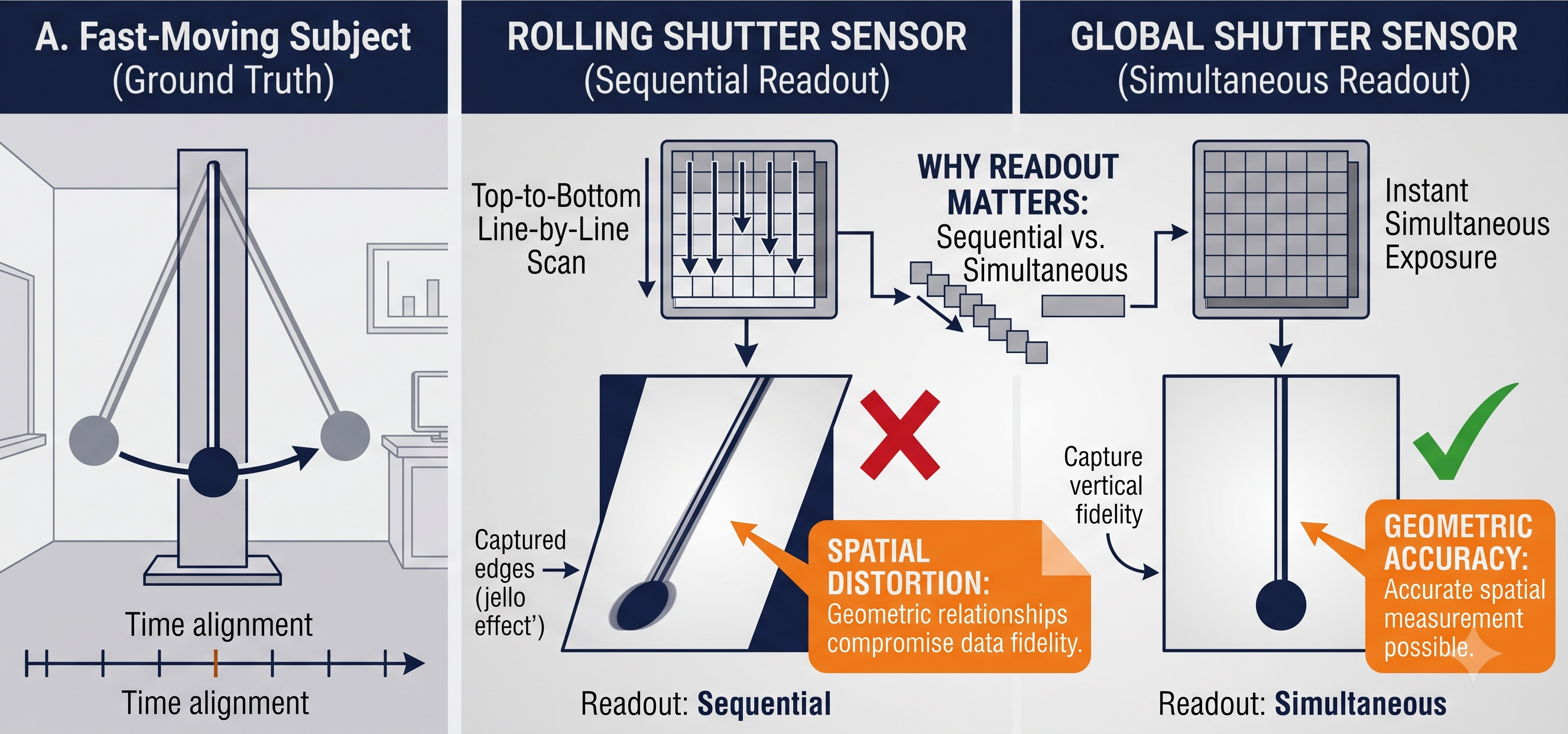
Figure 03: Key sensor properties in digital video. Physical size, photosite density, color versus monochrome design, and rolling versus global shutter behavior all shape what visual information can be recorded and how reliable that information will be for later analysis.
From Still Images to Video: Frames, Frame Rate, and Time
So far, we have described how a camera records a single image. Video begins when that process is repeated over and over again at controlled time intervals. A camera does not record motion directly as a separate substance. Instead, it records a rapid sequence of still images called frames. When those frames are arranged in order and played back quickly, we perceive continuous motion.
Each frame is a complete image with its own pixel grid, color values, and brightness information. What makes video different from a still image is not a new kind of pixel, but the addition of time. If a camera records 30 frames every second, then it is sampling the visible world 30 times per second. A short equation makes this intuitive:
For example, one minute of video recorded at 30 frames per second contains:
In Python terms, if a single color image can be thought of as an array with shape , then a video can be thought of conceptually as a time-ordered stack of such images, often represented like . This is one reason digital video is so useful for computation: it preserves not only appearance, but appearance changing over time.
The frame rate, measured in frames per second (fps), determines the temporal resolution of the video. A lower frame rate records fewer visual samples per second, whereas a higher frame rate records more. Common values such as 24 fps, 30 fps, 60 fps, and 120 fps do not simply change how smooth a video looks. They change how finely motion can be observed and measured. The time between consecutive frames is called the frame interval and is given by:
At 30 fps, one frame is recorded every 33.3 milliseconds. At 120 fps, one frame is recorded every 8.3 milliseconds. This difference matters when the event of interest is brief. A blink, a wing beat, a finger tap, or a rapid body turn may be only partially visible at 30 fps but much more clearly resolved at 120 fps.
Higher frame rates, however, are not free. Recording more frames per second increases the amount of data that must be stored and often reduces the amount of light available to each frame, especially when fast shutter speeds are also required. This is why frame rate, shutter speed, illumination, and sensor performance are tightly linked in practice. Choosing a frame rate is therefore not only a visual decision. It is also a measurement decision about how finely change through time must be sampled.
How Much Data Is in an Image or Video?
Once video is understood as a time-ordered stack of measured frames, a natural question follows: how much data does that actually create? The answer grows quickly, because every frame contains many pixels, every pixel can contain multiple channels, and video records many such frames every second.
For a raw digital image, a useful first approximation is:
For a 1920 by 1080 RGB image with 8 bits per channel, the raw size is:
That is equal to 6,220,800 bytes, or about 6.2 MB of raw image data before compression. If the image were grayscale instead of RGB, it would use only one channel rather than three, and the storage requirement would drop accordingly.
For raw video, the calculation extends across time:
If one minute of video is recorded at 1920 by 1080 resolution, in RGB color, with 8 bits per channel and 30 frames per second, then the raw data size is:
That is about 11.2 GB of raw video data for only one minute of recording. Higher resolution, higher frame rate, more channels, or greater bit depth all increase this value further. This is one reason video analysis can become computationally demanding very quickly: the amount of information grows along both spatial and temporal dimensions.
These calculations are intentionally simplified, but they are useful because they reveal the scale of the problem. A camera is not just recording what we see. It is generating a large numerical record of the scene, frame after frame, second after second.
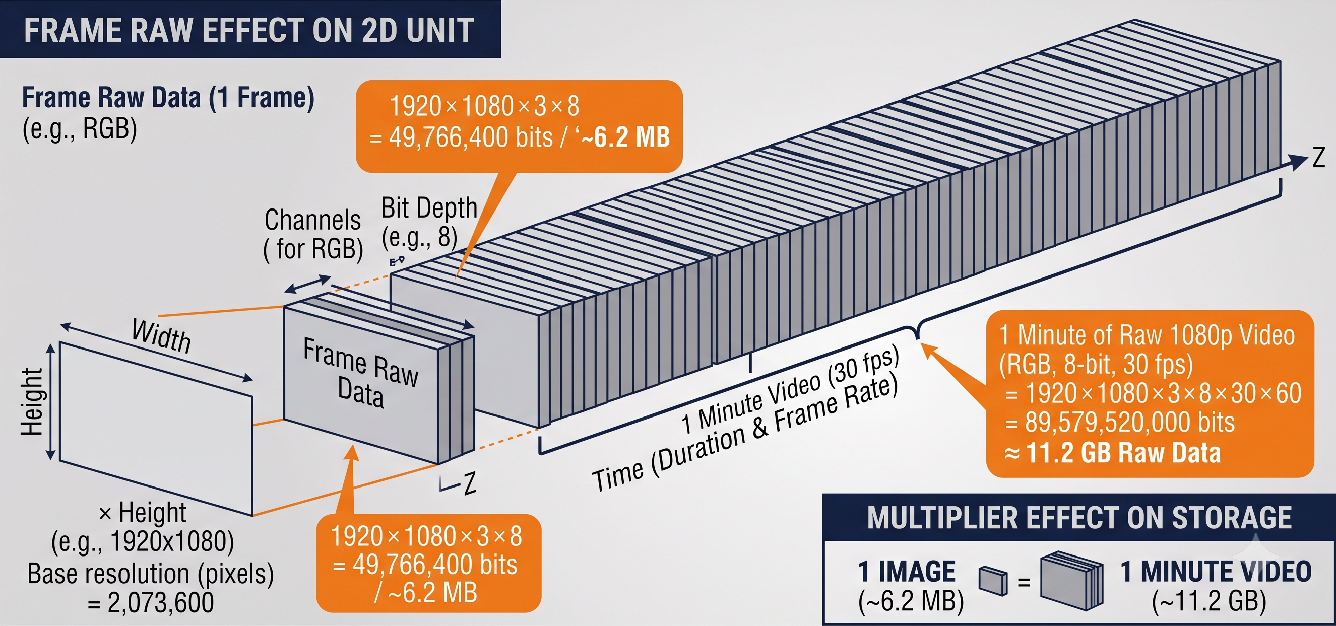
Figure 04: Raw image and video size grow from the combined effects of resolution, channel count, bit depth, frame rate, and duration. Video becomes large because it extends image data through time.
Compression, Codecs, and Why Video Files Are Smaller
If raw video becomes so large so quickly, why are everyday video files often far smaller than the calculations above suggest? The answer is compression. Most video is not stored as raw frame data. Instead, it is encoded so that repeated or less visually important information uses fewer bits.
At a basic level, compression works in two ways. First, it reduces redundancy within a frame by simplifying or encoding repeated visual patterns more efficiently. Second, it reduces redundancy across frames by storing changes over time rather than saving every frame as a completely independent image. A static background, for example, does not need to be fully rewritten 30 or 60 times every second if only one moving subject changes from frame to frame.
This distinction helps explain why a video file is not simply a folder full of images. Some frames may be stored more completely, while many others are stored mainly as differences relative to nearby frames. That strategy can reduce file size dramatically, but it also means that the stored video is already a processed version of the original measurements.
Two terms are especially useful here:
Codec: The method used to compress and decompress video data. Common examples include H.264, H.265, and AV1.
Container: The file wrapper that holds the encoded video, and often audio and metadata as well. Common examples include MP4, MOV, and MKV.
This is why two files with the same duration and resolution can behave very differently. An MP4 file does not tell us exactly how the video was compressed; it tells us mainly about the container. The underlying codec, bitrate, color handling, and compression strength all influence image quality, file size, and usefulness for later analysis.
Compression can be lossless or lossy. Lossless compression preserves all original information and simply stores it more efficiently. Lossy compression permanently removes some information to make files much smaller. Many everyday video formats are lossy, and they often reduce fine detail, smooth subtle textures, or simplify color information more aggressively than brightness information. For casual viewing this may be acceptable. For scientific measurement, it can matter a great deal.
This is especially important in behavioral research. If the goal is only to watch a recording, strong compression may be perfectly adequate. But if the goal is to measure tiny movements, detect subtle posture changes, or track features frame by frame, compression artifacts can interfere with the data. A file that looks visually acceptable to a human observer may still be less reliable for computational analysis.
For that reason, video literacy includes more than knowing how to record footage. It also includes understanding how that footage has been encoded, what information may have been discarded, and whether the resulting file is suitable for the scientific question at hand.
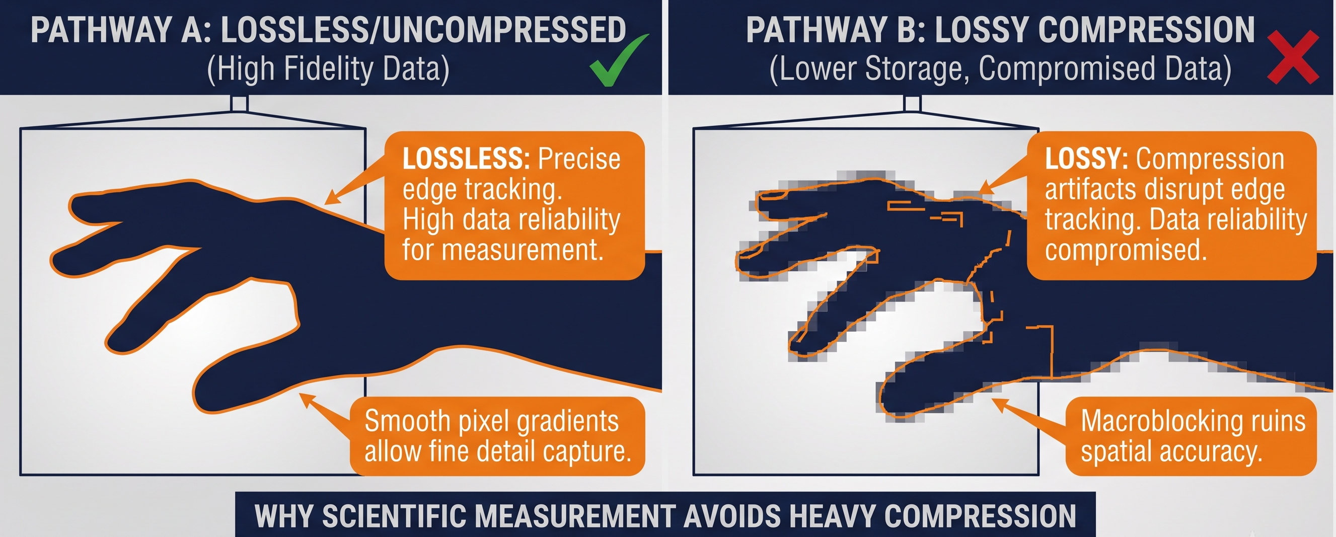
Figure 05: Compressed video files are smaller than raw frame data because codecs reduce redundancy within and across frames. Containers such as MP4 or MOV hold the encoded video stream, but the codec determines how the data has actually been stored.
From Video to Behavioral Data
Videos store a time-ordered record of light, color, shape, and motion. Behavioral data emerges when that visual record is examined with a clear research question and converted into measurable variables.
This transformation can happen at several levels. At the simplest level, a researcher may watch a recording and annotate events manually: when an animal enters a zone, when a person smiles, when a hand gesture begins, or how long two individuals remain close to one another. In that case, the video serves as a replayable record from which behavioral observations can be coded. This is also how many classic studies of behavior were conducted using film recordings: researchers repeatedly watched recorded scenes and coded events, durations, and action sequences by hand.
However, with digital videos, we can computationally perform quite a lot of tasks using the structured measurements. A program can compare frames to estimate motion, detect objects with certain features, track the position of a body across time, detect landmarks such as joints or facial features, or measure distances between individuals and objects. From those visual measurements, researchers can derive behavioral variables such as trajectory, speed, posture, orientation, proximity, synchrony, or event timing.
This is an important conceptual shift. Pixels, frames are not behaviors. Even motion itself is not yet behavior in an interpretive sense. They are measurements from which behavior may be inferred. A person leaning forward, an animal freezing, or a group moving together becomes behavioral data only when the recorded visual patterns are linked to a defined analytic question.
For that reason, good behavioral video analysis depends on more than software alone. It depends on whether the video preserves the information needed for the research goal. If frame rate is too low, a brief action may be missed. If compression is too strong, subtle movement may be blurred or simplified. If lighting is poor, tracking may fail. If the camera angle is poorly chosen, key body parts may be hidden. The quality of behavioral data is therefore shaped long before any analysis begins.
This is also why digital video has become so powerful in scientific research. Once motion is stored as measurable visual data, researchers are no longer limited to memory or impression. They can revisit events, quantify patterns, compare observations across coders, and build reproducible workflows that connect recording, analysis, and interpretation.
In the next guide, we will take the next step in that transformation by examining how computers analyze video more directly through computer vision. There, the question will no longer be only how video is recorded, but how visual data can be detected, tracked, and transformed into meaningful behavioral measurements.