Authored by Souvik Mandal, Ph.D.
Project Leader & Instructor, Computational Behavioral Sciences, LS100, FAS, Harvard University | Linkedin ID: souvik-mandal-phd
Last updated: 2026-07-02


Step 0. Setup
# Please make sure to install the required libraries. You can do this by running the
# %pip install <library-name>
# command in a Jupyter notebook cell. Below are the libraries you need for this notebook.

# %pip install -q librosa soundfile # For audio processing
# %pip install -q matplotlib seaborn plotly # For data visualization
# %pip install "nbformat>=4.2.0" # Required for Jupyter notebook compatibility
# %pip install ipywidgets # For interactive widgets (optional, but useful for audio playback)
from pathlib import Path
import numpy as np
import pandas as pd
import librosa, librosa.display
import re
import sys
print(sys.executable)/Users/souvikmandal/anaconda3/envs/Analysis_Engineering/bin/python
# --- Global plot configuration (applies to all figures) ---
import matplotlib.pyplot as plt
import seaborn as sns

sns.set_theme(style="whitegrid", context="notebook", palette="muted")

# Plot configuration that applies to all figures
plt.rcParams.update({
    "figure.figsize": (10, 3),        # fixed size for all figures
    "axes.titlesize": 13,
    "axes.labelsize": 11,
    "axes.grid": True,
    "grid.alpha": 0.3,
    "grid.linestyle": "--",
    "axes.facecolor": "#f9f9f9",
    "figure.facecolor": "white",
})

sns.set_theme(style="darkgrid", context="notebook", palette="muted")

# Setting up Plotly

import plotly
import plotly.io as pio
import plotly.graph_objects as go
import plotly.express as px

print("plotly version:", plotly.__version__)
print("current default renderer:", repr(pio.renderers.default))
print("available renderers:", list(pio.renderers.keys())[:10], "...")

# Prefer modern inline renderer; fall back to iframe if needed
try:
    pio.renderers.default = "notebook_connected"
except Exception:
    pio.renderers.default = "iframe"

print("\nUsing plotly renderer:", pio.renderers.default)
plotly version: 6.8.0
current default renderer: 'vscode'
available renderers: ['plotly_mimetype', 'jupyterlab', 'nteract', 'vscode', 'notebook', 'notebook_connected', 'kaggle', 'azure', 'colab', 'cocalc'] ...
Using plotly renderer: notebook_connected
# Test figure for Plotly
x = np.linspace(0, 2*np.pi, 200)
y = np.sin(x)

fig = go.Figure()
fig.add_scatter(x=x, y=y, mode="lines", name="sine")
fig.update_layout(title="Plotly test figure")
fig.show()
Step 1.0. Load one audio file and visualize the waveform
We’ll start by loading a single track; paste the location of the track below.
from pathlib import Path

audio_path = Path("/Users/souvikmandal/Documents/S06_Teaching_Mentoring_Talks/LS100/av_media_files/audio/music_tracks/Eagles_Hotel-California.mp3")

print(f"Does {audio_path.name} exist? {audio_path.is_file()}")
Now, let’s plot its waveform.
The waveform shows how amplitude (loudness) changes over time.
What are we loading - the y and sr? (click to expand)
When we load an audio file with librosa, we usually write:
y, sr = librosa.load(audio_path, sr=None) # librosa loads the track as mono by default. You can add `mono=True/ False` after sr=None.Here’s what each variable means:
| Variable | Meaning | In simple words | Example |
|---|---|---|---|
y | The audio time series | A long list (NumPy array) of numbers representing the waveform — how air pressure changes over time. Each value is a tiny snapshot of loudness. | [-0.0021, 0.0053, 0.0089, ...] |
sr | The sampling rate (in Hz) | How many of those numbers are recorded per second. Typical values are 44,100 Hz (CD quality) or 48,000 Hz (studio standard). | 44100 |
Additional notes:
If you load mono,
yhas shape(n_samples,).If you load stereo,
yhas shape(2, n_samples)— one row per channel (Left, Right).You can compute duration easily:
duration_sec = len(y) / sr
print(f"Duration: {duration_sec:.2f} seconds")
if audio_path.exists():
    y, sr = librosa.load(audio_path, sr=None)
    duration_sec = len(y) / sr
    print(f"Loaded: {audio_path.name}")
    print("Sample rate:", sr, "Hz  |  Samples:", len(y), "  |  Duration:", round(duration_sec, 2), "s")
else:
    print("No audio file loaded. Please set audio_path to a valid .wav or .mp3 file.")
    y, sr = None, None

if y is not None:
    sns.set_style("darkgrid")
    plt.figure()
    librosa.display.waveshow(y, sr=sr, color=sns.color_palette("muted")[0], alpha=0.8)
    plt.title("Waveform", fontsize=13, fontweight="bold")
    plt.xlabel("Time (s)")
    plt.ylabel("Amplitude")
    sns.despine()
    plt.show()
Loaded: Eagles_Hotel-California.mp3
Sample rate: 44100 Hz  |  Samples: 11438208   |  Duration: 259.37 s
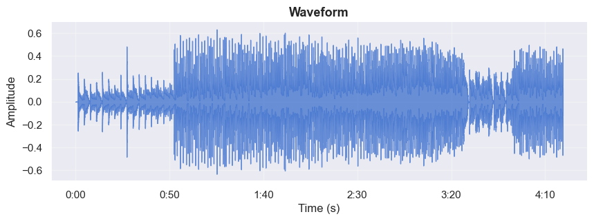
If you want an interactive plot for the waveform, run the following code bock.
# --- Interactive waveform (Plotly) ---
#Used packages/ modules: numpy as np; plotly.graph_objects as go

if y is not None:
    # Time axis
    t = np.arange(len(y)) / sr

    # Lightweight downsampling for interactivity (aim ~5k points)
    target_pts = 5000
    step = max(1, len(y) // target_pts)
    t_ds = t[::step]
    y_ds = y[::step]

    fig = go.Figure()

    fig.add_trace(
        go.Scatter(
            x=t_ds,
            y=y_ds,
            mode="lines",
            line=dict(width=1.2),
            name="Waveform",
            hovertemplate="t = %{x:.2f}s<br>amp = %{y:.3f}<extra></extra>",
        )
    )

    fig.update_layout(
        title=dict(text="Waveform (Interactive)", x=0.5),
        xaxis=dict(
            title="Time (s)",
            rangeselector=dict(
                buttons=list([
                    dict(count=5, label="5s", step="second", stepmode="backward"),
                    dict(count=30, label="30s", step="second", stepmode="backward"),
                    dict(step="all")
                ])
            ),
            rangeslider=dict(visible=True),
            type="linear",
            showgrid=True,
            zeroline=False,
        ),
        yaxis=dict(
            title="Amplitude",
            showgrid=True,
            zeroline=False,
        ),
        height=300,
        margin=dict(l=60, r=30, t=60, b=50),
        hovermode="x unified",
        showlegend=False,
    )

    fig.show()
else:
    print("Please load an audio file first (see Step 1).")
Step 2 — From Waveform to Frequency: The Discrete Fourier Transform (DFT)
Now that we’ve seen what the audio looks like as a waveform — amplitude changing over time — let’s explore what frequencies make up that sound.
We can take the full track or a short slice of the waveform and compute its Discrete Fourier Transform (DFT) to reveal its frequency components.
The DFT answers the question: “What notes or tones are present in this track (or at a particular moment of it)?”
2.1 The Full-Track DFT
If we take the DFT of the entire song, we get the overall frequency content — a kind of “fingerprint” of all tones and harmonics that ever occur.
For example, it might show that there’s a strong 440 Hz tone (A4) somewhere in the track.
However:
It tells us what frequencies are present,
but not when they occur.
Everything is merged together into a single global spectrum.
Understanding the Y-Axis (in Decibels)
The vertical axis shows magnitude — the strength of each frequency component — but it’s measured in decibels (dB) instead of raw amplitude.
That’s why you see negative values on the y-axis.
| Concept | Explanation |
|---|---|
| Reference (0 dB) | The loudest frequency in the entire track. It’s the peak amplitude. |
| Negative values (e.g., –20 dB, –60 dB) | Frequencies that are quieter than the loudest one. For instance, –20 dB means 10× quieter; –60 dB means 1000× quieter. |
| Why use dB? | The decibel scale matches how human hearing perceives loudness — logarithmically — and it compresses a huge dynamic range into a readable plot. |
.
In simple terms:
0 dB = loudest tone,
–80 dB = much quieter tone,
but all values are still positive in energy — “negative dB” just means “quieter than the loudest frequency.”
Next, we’ll visualize this DFT interactively and overlay typical instrument frequency bands (bass, vocals, cymbals, etc.) to understand where each part of the mix lives in the spectrum.
# --- Step 2.1: Global DFT with instrument bands (Plotly; no overlaps, legend outside right) ---
import numpy as np
import plotly.graph_objects as go
import plotly.express as px

if y is None:
    print("Please load an audio file in Step 1 first.")
else:
    # ----- Compute full-track DFT -----
    N = len(y)
    Y = np.fft.rfft(y)
    freqs = np.fft.rfftfreq(N, d=1/sr)
    mag = np.abs(Y)
    mag_db = 20 * np.log10(np.maximum(mag, 1e-12) / np.max(mag))

    # Focus range
    fmin, fmax = 20.0, 20000.0
    use = (freqs >= fmin) & (freqs <= fmax)
    freqs_use = freqs[use]
    mag_db_use = mag_db[use]

    # Downsample for interactivity (log-spaced)
    n_bins = 2000
    bins = np.geomspace(fmin, fmax, n_bins + 1)
    which_bin = np.digitize(freqs_use, bins) - 1
    pooled_f, pooled_db = [], []
    for b in range(n_bins):
        mask = which_bin == b
        if np.any(mask):
            f_left, f_right = bins[b], bins[b + 1]
            pooled_f.append(np.sqrt(f_left * f_right))
            pooled_db.append(np.max(mag_db_use[mask]))
    pooled_f = np.asarray(pooled_f, float)
    pooled_db = np.asarray(pooled_db, float)

    peak_db = float(np.nanmax(pooled_db))
    y_min, y_max = peak_db - 80.0, peak_db + 3.0

    # Band definitions
    bands = [
        {"label": "Bass & Kick Drum",       "range": (20,   250),  "color": "#fde725", "alpha": 0.20},
        {"label": "Vocals, Guitars, Snare", "range": (250,  5000), "color": "#55c667", "alpha": 0.15},
        {"label": "Cymbals & Air",          "range": (5000, 20000),"color": "#3b528b", "alpha": 0.12},
    ]

    fig = go.Figure()

    # Spectrum line
    fig.add_trace(
        go.Scatter(
            x=pooled_f, y=pooled_db, mode="lines",
            line=dict(width=1.3, color=px.colors.qualitative.Plotly[0]),
            name="Magnitude (dB, ref max)",
            hovertemplate="f = %{x:.1f} Hz<br>dB = %{y:.1f}<extra></extra>",
        )
    )

    # Add shaded bands as shapes (no legend, never overlap labels)
    for b in bands:
        fig.add_vrect(
            x0=b["range"][0], x1=b["range"][1],
            fillcolor=b["color"], opacity=b["alpha"],
            line_width=0, layer="below"
        )

    # Add dummy legend items for the bands (no data plotted)
    for b in bands:
        fig.add_trace(
            go.Scatter(
                x=[None], y=[None],
                mode="markers",
                marker=dict(size=10, color=b["color"]),
                name=b["label"],
                hoverinfo="skip",
                showlegend=True,
            )
        )

    # Layout: legend outside on the right, extra right margin, no overlaps
    fig.update_layout(
        title=dict(text="Global Magnitude Spectrum with Instrument Frequency Bands", x=0.5),
        xaxis=dict(
            title="Frequency (Hz)",
            type="log",
            range=[np.log10(fmin), np.log10(fmax)],
            showgrid=True, zeroline=False
        ),
        yaxis=dict(
            title="Magnitude (dB, ref max)",
            range=[y_min, y_max],
            showgrid=True, zeroline=False
        ),
        height=360,
        margin=dict(l=60, r=200, t=70, b=60),   # <- make room for right-side legend
        legend=dict(
            orientation="v",
            xanchor="left", x=1.02,              # <- outside right
            yanchor="top",  y=1.0,
            bgcolor="rgba(255,255,255,0.85)",
            bordercolor="rgba(0,0,0,0.15)",
            borderwidth=1,
            font=dict(size=11)
        ),
        hovermode="x unified"
    )

    # Prevent label clipping
    fig.update_xaxes(automargin=True)
    fig.update_yaxes(automargin=True)
    fig.add_annotation(x=100,  y=-10, text="Bass & Kick Drum", showarrow=False, font=dict(size=11))
    fig.add_annotation(x=1000, y=-10, text="Vocals, Guitars, Snare", showarrow=False, font=dict(size=11))
    fig.add_annotation(x=10000, y=-10, text="Cymbals & Air", showarrow=False, font=dict(size=11))


    print(f"Track length: {N:,} samples  |  Duration: {N/sr:.2f} s")
    print(f"Frequency resolution: {sr/N:.4f} Hz per bin")

    fig.show()
Track length: 11,438,208 samples  |  Duration: 259.37 s
Frequency resolution: 0.0039 Hz per bin
2.2. The short-slice (windowed) DFT
Music constantly changes — new notes, instruments, and beats appear over time.
To capture this evolution, we take a short slice of the waveform (for example, 1 second).
The DFT of this slice shows the frequencies active at that specific moment.
Repeating this for overlapping slices across time produces a spectrogram — a visual record of how the frequency content changes through the song.
The time–frequency trade-off
| Window Length | Frequency Resolution | Time Resolution | When to Use |
|---|---|---|---|
| Long window | Precise frequency details | Blurry timing | For stable, steady notes |
| Short window | Less precise frequencies | Better timing accuracy | For fast-changing sounds or rhythms |
.
Tip: Start with ~1 second, then try shorter/longer and watch the peaks sharpen or blur.
# DEFINE AT WHAT POINT OF TIME YOU WANT TO ANALYZE THE SPECTRUM
center_t = 30.0   # seconds
slice_sec = 1.0   # seconds (try 0.5, 2.0, ...)
# --- Step 2.2: One-slice DFT (interactive, Plotly) ---
# Used packages/modules: numpy as np; plotly.graph_objects as go
if y is None:
print("Please load an audio file in Step 1 first.")
else:
# ---- pick the slice (kept inside file bounds) ----
duration_sec = len(y) / sr
center_t = float(np.clip(center_t, slice_sec/2, max(slice_sec/2, duration_sec - slice_sec/2)))
i0 = int(round((center_t - slice_sec/2) * sr))
i1 = i0 + int(round(slice_sec * sr))
x = y[i0:i1]
if len(x) < 4:
print("Audio slice too short to analyze.")
else:
# ---- window + zero-pad to next power of 2, then FFT ----
w = np.hanning(len(x))
xw = x * w
N = int(2 ** np.ceil(np.log2(len(xw)))) # next power of 2
X = np.fft.rfft(xw, n=N)
f = np.fft.rfftfreq(N, d=1.0/sr)
mag = np.abs(X)
mag_db = 20.0 * np.log10(np.maximum(mag, 1e-12) / (np.max(mag) + 1e-12))
delta_f = sr / N
print(f"Slice center: {center_t:.2f}s | Window: {len(x)} samples | N_fft: {N} | Δf ≈ {delta_f:.2f} Hz")
# ---- pick top K well-separated peaks for markers ----
K = 5
low_hz = 100.0
idx_ok = np.where(f >= low_hz)[0]
if idx_ok.size:
# take many candidates then enforce spacing
cand = idx_ok[np.argsort(mag[idx_ok])[-(K*6):]] # more than K
cand = cand[np.argsort(mag[cand])[::-1]] # sort by strength
marked = []
for k in cand:
if all(abs(f[k] - f[j]) > 30 for j in marked): # ≥30 Hz apart
marked.append(k)
if len(marked) >= K:
break
else:
marked = []
# ---- dynamic y-range (~80 dB window) ----
peak_db = float(np.nanmax(mag_db))
y_min, y_max = peak_db - 80.0, peak_db + 3.0
# ---- build Plotly figure ----
fig = go.Figure()
# main spectrum line
fig.add_trace(go.Scatter(
x=f, y=mag_db, mode="lines",
line=dict(width=1.3),
name="Magnitude (dB, ref max)",
hovertemplate="f = %{x:.1f} Hz<br>dB = %{y:.1f}<extra></extra>",
))
# vertical markers for peaks
for k in marked:
fig.add_vline(
x=float(f[k]), line_width=1, line_dash="dash", line_color="gray",
annotation_text=f"{int(f[k])} Hz", annotation_position="top right",
annotation_font=dict(size=10, color="gray")
)
# layout: log x-axis, slider, compact margins
fig.update_layout(
title=dict(text="One-Slice Magnitude Spectrum (DFT, dB)", x=0.5),
xaxis=dict(
title="Frequency (Hz)",
type="log",
range=[np.log10(max(20, f[1] if len(f) > 1 else 20)), np.log10(sr/2)],
rangeslider=dict(visible=False),
showgrid=True, zeroline=False
),
yaxis=dict(
title="Magnitude (dB, ref max in slice)",
range=[y_min, y_max],
showgrid=True, zeroline=False
),
height=300,
margin=dict(l=60, r=30, t=60, b=50),
hovermode="x unified",
showlegend=False
)
fig.show()
Slice center: 30.00s | Window: 44100 samples | N_fft: 65536 | Δf ≈ 0.67 Hz
2.3. Spectrogram: Frequencies Changing Over Time
A spectrogram shows how sound energy is distributed across frequency as the music progresses in time.
| Axis | Represents | Description |
|---|---|---|
| X-axis | Time | Moves left → right as the song plays |
| Y-axis | Frequency | Low notes at the bottom, high notes at the top |
| Color (intensity) | Amplitude (loudness) | Brighter areas mean stronger energy at that frequency |
.
Think of it as: DFT on many short, overlapping slices → stack the spectra → color by strength.
Explore before coding:
Try this interactive website to see how different sounds look in a spectrogram:
👉 musiclab
💡 A spectrogram is like a thermal camera for sound:
Horizontal bands often correspond to sustained harmonics — vocals, guitar, or synths.
Vertical bursts usually represent transients — drum hits or sharp attacks.
How we compute the spectrogram (and why use the Mel scale + dB) (click to expand)
To build a spectrogram, we:
Slice the audio into overlapping windows.
Compute a Short-Time Fourier Transform (STFT) for each window to find the active frequencies.
Stack all slices together in time order — this becomes the spectrogram.
There are two common types:
STFT spectrogram → frequencies in Hz (raw physical values).
Mel-spectrogram → frequencies warped to match human hearing (dense in lows, sparse in highs).
We’ll use a Mel-spectrogram because:
It mirrors how the ear perceives pitch.
It focuses resolution where it matters most for music — bass, vocals, and midrange.
It converts energy to decibels (dB) using
power_to_db, making quiet details visible.
| Parameter | Effect | When to Adjust |
|---|---|---|
n_fft | Larger = better frequency resolution, blurrier time | Long sustained tones |
hop_length | Smaller = finer time resolution, more frames | Percussive or fast passages |
n_mels | More Mel bands = smoother detail | Rich harmonic music |
We’ll keep hop_length consistent with earlier steps so that time axes align across plots.
# --- Step 2.3: Mel-Spectrogram (interactive, Plotly) ---
# Uses: numpy as np; librosa; plotly.graph_objects as go

if y is None:
    print("Please load an audio file in Step 1 first.")
else:
    # Parameters (feel free to experiment)
    n_fft = 2048
    hop_length = 512          # keep consistent with earlier steps
    n_mels = 128
    fmin, fmax = 20.0, sr/2   # Mel range

    # Mel-spectrogram (power) -> dB
    S = librosa.feature.melspectrogram(
        y=y, sr=sr, n_fft=n_fft, hop_length=hop_length,
        n_mels=n_mels, fmin=fmin, fmax=fmax, power=2.0
    )
    S_db = librosa.power_to_db(S, ref=np.max)

    # Axes
    times = librosa.frames_to_time(np.arange(S_db.shape[1]), sr=sr, hop_length=hop_length)
    mel_freqs_hz = librosa.mel_frequencies(n_mels=n_mels, fmin=fmin, fmax=fmax)

    # Dynamic Z range (~80 dB window for contrast)
    zmax = float(np.nanmax(S_db))
    zmin = zmax - 80.0

    # Build interactive heatmap
    fig = go.Figure(
        data=go.Heatmap(
            x=times,
            y=mel_freqs_hz,        # show y in Hz even though spacing is Mel
            z=S_db,
            colorscale="Magma",
            zmin=zmin, zmax=zmax,
            colorbar=dict(title="dB")
        )
    )

    # Nice ticks for log-frequency
    tick_vals = [50, 100, 200, 500, 1000, 2000, 5000, 10000, min(20000, int(sr/2))]
    tick_vals = [v for v in tick_vals if fmin <= v <= fmax]

    fig.update_layout(
        title=dict(text="Mel-Spectrogram (dB)", x=0.5),
        xaxis=dict(
            title="Time (s)",
            rangeslider=dict(visible=True),   # zoom with slider
            showgrid=True, zeroline=False
        ),
        yaxis=dict(
            title="Frequency (Hz, Mel-spaced)",
            type="log",                       # log display for intuitive reading
            tickmode="array",
            tickvals=tick_vals,
            ticktext=[f"{v//1000}k" if v>=1000 else f"{v}" for v in tick_vals],
            showgrid=True, zeroline=False
        ),
        height=320,
        margin=dict(l=70, r=40, t=60, b=60),
    )

    # Hover shows time, freq, and dB
    fig.update_traces(
        hovertemplate="t = %{x:.2f}s<br>f = %{y:.0f} Hz<br>level = %{z:.1f} dB<extra></extra>"
    )

    fig.show()
Step 3. Extract Tempo, Beats, and Rhythm Structure
Now that we can visualize how sound changes across frequencies, let’s focus on the time structure of the music —
its tempo (speed), beat pattern, and rhythmic flow.
These rhythmic features form the backbone of most musical tracks:
Tempo (BPM) → how fast the music is.
Beats → the recurring pulses you could tap your foot to.
Downbeats and rhythm structure → how beats group into measures (the musical “grid”).
3.1 : Tempo, Beats
In this step, we’ll use librosa to detect:
The global tempo of the track (in Beats Per Minute, or BPM),
The positions of beats over time,
The local tempo curve — how the rhythm evolves or fluctuates across the song.
How does a computer detect rhythm — and can a song have multiple tempos? (click to expand)
Humans sense rhythm intuitively — we tap our foot or nod along.
Computers must analyze the waveform to find repeating energy patterns, then estimate the timing of those pulses.
Here’s the step-by-step idea:
Onset Detection:
The program measures sudden changes in loudness or energy.
Each spike (called an onset) marks the beginning of a sound event — like a drum hit or chord.Beat and Tempo Estimation:
By looking at how often onsets occur, we can estimate the tempo (beats per minute, or BPM).
Most songs have one clear tempo, but some can contain multiple dominant tempos —
for example, a halftime or double-time section, or a brief tempo shift during a solo.Dominant BPMs:
By aggregating tempo energy across time, we can identify one or more dominant tempos that the song tends to revolve around.
Each dominant BPM shows a stable rhythmic “mode” of the track.Rhythm Structure:
Once beats are identified, we can map how tempo evolves — this reveals performance dynamics,
such as small accelerations, slowdowns, or expressive rubato.
Key takeaway:
A steady pop song will typically have one strong dominant BPM,
while more complex or live performances can show two or more rhythmic modes.
# --- Step 3.1 : Tempo, Beats (with dominant BPM summary) ---
# Uses: numpy as np, librosa, plotly.graph_objects as go

if y is None:
    print("Please load an audio file in Step 1 first.")
else:
    hop_length = 256  # keep consistent across steps

    # ===== 1) Global tempo + beats =====
    tempo_bpm, beat_frames = librosa.beat.beat_track(y=y, sr=sr, hop_length=hop_length)
    tempo_bpm_scalar = float(np.atleast_1d(tempo_bpm)[0])
    beat_times = librosa.frames_to_time(beat_frames, sr=sr, hop_length=hop_length)

    # Instantaneous BPM from beat intervals
    if len(beat_times) >= 2:
        ibi = np.diff(beat_times)                      # seconds
        inst_bpm = 60.0 / ibi                          # BPM per interval
        inst_times = 0.5 * (beat_times[1:] + beat_times[:-1])
    else:
        inst_bpm = np.array([])
        inst_times = np.array([])

    # ===== 2) Dominant tempo(s) via time-averaged tempogram =====
    onset_env = librosa.onset.onset_strength(y=y, sr=sr, hop_length=hop_length)
    tg = librosa.feature.tempogram(onset_envelope=onset_env, sr=sr, hop_length=hop_length)
    tempi = librosa.tempo_frequencies(tg.shape[0], sr=sr, hop_length=hop_length)  # BPM bins
    profile = np.mean(tg, axis=1)

    # simple peak picking with threshold
    thresh = 0.20 * np.max(profile) if np.max(profile) > 0 else 0.0
    peaks_idx = []
    for i in range(1, len(profile) - 1):
        if profile[i] >= profile[i - 1] and profile[i] >= profile[i + 1] and profile[i] >= thresh:
            peaks_idx.append(i)
    dominant_bpms = tempi[peaks_idx]

    # Group instantaneous BPMs around each dominant BPM (±6% tolerance); drop zero-support bins
    tol_frac = 0.06
    records = []
    for bpm0 in dominant_bpms:
        if inst_bpm.size == 0:
            support_mask = np.array([], dtype=bool)
        else:
            tol = tol_frac * bpm0
            support_mask = (inst_bpm >= bpm0 - tol) & (inst_bpm <= bpm0 + tol)
        support_intervals = int(np.sum(support_mask))
        approx_beats = support_intervals + 1 if support_intervals > 0 else 0
        if approx_beats == 0:
            continue  # drop bins with zero beat support
        est_tempo = float(np.median(inst_bpm[support_mask])) if support_intervals > 0 else float(bpm0)
        records.append({
            "dominant_bpm_bin": float(bpm0),
            "estimated_tempo_bpm": round(est_tempo, 1),
            "supporting_intervals": support_intervals,
            "approx_beats": approx_beats
        })

    # Fallback: if nothing survives, use global tempo as sole record
    if len(records) == 0:
        records = [{
            "dominant_bpm_bin": float(tempo_bpm_scalar),
            "estimated_tempo_bpm": round(tempo_bpm_scalar, 1),
            "supporting_intervals": int(len(inst_bpm)),
            "approx_beats": int(len(inst_bpm) + 1 if len(inst_bpm) > 0 else len(beat_times))
        }]

    allow_outlier_filter = (len(records) <= 1)

    # Console summary
    print(f"Estimated global tempo (track-level): {tempo_bpm_scalar:.1f} BPM")
    print(f"Detected beats (total): {len(beat_times)}")
    print("\nDominant tempo(s) and support:")
    for r in records:
        print(f"  • Bin ≈ {r['dominant_bpm_bin']:.1f} BPM  |  "
              f"Estimated: {r['estimated_tempo_bpm']:.1f} BPM  |  "
              f"Supporting intervals: {r['supporting_intervals']}  |  "
              f"~Beats: {r['approx_beats']}")
    print(f"\nOutlier filtering (±2 SD) allowed in this track?  {allow_outlier_filter}")

    # ===== 3) Local tempo curve (weighted tempogram + fallback) =====
    times = librosa.frames_to_time(np.arange(tg.shape[1]), sr=sr, hop_length=hop_length)

    col_sums = np.sum(tg, axis=0)
    with np.errstate(divide="ignore", invalid="ignore"):
        weighted_tempo = np.sum(tg * tempi[:, None], axis=0) / np.where(col_sums == 0, np.nan, col_sums)

    if inst_bpm.size > 0:
        inst_on_grid = np.interp(times, inst_times, inst_bpm, left=inst_bpm[0], right=inst_bpm[-1])
    else:
        inst_on_grid = np.full_like(times, np.nan, dtype=float)

    local = weighted_tempo.astype(float)
    local[~np.isfinite(local)] = np.nan
    need_fallback = np.isnan(local)
    if np.any(need_fallback):
        local[need_fallback] = inst_on_grid[need_fallback]
    local[np.isnan(local)] = tempo_bpm_scalar  # final safety

    # smoothing
    def moving_average(x, window=40):
        x = np.asarray(x, float)
        if window < 2 or len(x) < window:
            return x
        kernel = np.ones(window, dtype=float) / window
        return np.convolve(x, kernel, mode="same")

    local_smooth = moving_average(local, window=15)

    # ===== 4) Optional ±2 SD cleanup (only if single dominant tempo) =====
    if allow_outlier_filter and np.isfinite(local_smooth).any():
        mean_bpm = np.nanmean(local_smooth)
        std_bpm = np.nanstd(local_smooth)
        mask = (local_smooth < mean_bpm - 2 * std_bpm) | (local_smooth > mean_bpm + 2 * std_bpm)
        n_out = int(np.sum(mask))
        if n_out > 0:
            print(f"Filtered {n_out} local tempo outliers (>2 SD from mean).")
            local_smooth[mask] = np.nan
            idx = np.arange(len(local_smooth))
            good = np.isfinite(local_smooth)
            if np.sum(good) > 3:
                local_smooth = np.interp(idx, idx[good], local_smooth[good])

    # ===== 5) Auto-compact y-axis from robust quantiles =====
    vals = [local_smooth[np.isfinite(local_smooth)]]
    if inst_bpm.size > 0:
        vals.append(inst_bpm[np.isfinite(inst_bpm)])
    vals.append(np.array([tempo_bpm_scalar], dtype=float))
    vals = np.concatenate([v for v in vals if v.size > 0])

    if vals.size:
        q_lo, q_hi = np.nanpercentile(vals, [2, 100])
        pad = max(2.0, 0.1 * (q_hi - q_lo))
        y_min, y_max = q_lo - pad, q_hi + pad
        if (y_max - y_min) < 10:
            center = float(np.nanmedian(vals))
            y_min, y_max = center - 6, center + 6
    else:
        y_min, y_max = tempo_bpm_scalar - 6, tempo_bpm_scalar + 6

    # ===== 6) Plotly: Instantaneous BPM (beats) + Local Tempo (smoothed) =====
    fig = go.Figure()

    if inst_bpm.size > 0:
        fig.add_trace(go.Scatter(
            x=inst_times, y=inst_bpm,
            mode="markers",
            marker=dict(size=5, opacity=0.55),
            name="Instantaneous BPM (beats)",
            hovertemplate="t = %{x:.2f}s<br>BPM = %{y:.1f}<extra></extra>"
        ))

    fig.add_trace(go.Scatter(
        x=times, y=local_smooth,
        mode="lines",
        line=dict(width=1.6),
        name="Local Tempo (smoothed)",
        hovertemplate="t = %{x:.2f}s<br>BPM = %{y:.1f}<extra></extra>"
    ))

    fig.add_hline(
        y=tempo_bpm_scalar,
        line_width=1, line_dash="dash", line_color="gray",
        annotation_text=f"Global Tempo ≈ {tempo_bpm_scalar:.1f} BPM",
        annotation_position="top left"
    )

    total_duration = len(y) / sr
    fig.update_layout(
        title=dict(text="Tempo & Rhythm Structure", x=0.5),
        xaxis=dict(title="Time (s)", range=[0, total_duration], showgrid=True, zeroline=False),
        yaxis=dict(title="Tempo (BPM)", range=[y_min, y_max], showgrid=True, zeroline=False),
        height=320,
        margin=dict(l=70, r=40, t=60, b=60),
        hovermode="x unified",
        legend=dict(orientation="h", yanchor="bottom", y=1.02, xanchor="right", x=1.0)
    )

    fig.show()
Estimated global tempo (track-level): 147.7 BPM
Detected beats (total): 635

Dominant tempo(s) and support:
  • Bin ≈ 147.7 BPM  |  Estimated: 147.7 BPM  |  Supporting intervals: 604  |  ~Beats: 605

Outlier filtering (±2 SD) allowed in this track?  True
Filtered 1712 local tempo outliers (>2 SD from mean).
3.2 — Rhythm Structure (Musical Meter, e.g., 4/4, 3/4, 6/8)
Beyond tempo and beats, most music groups beats into repeating patterns called meter (or time signature).
Examples: 4/4 (four beats per bar), 3/4 (waltz feel), 6/8 (two big pulses, each subdivided into three).
We can estimate meter by looking for accent patterns across beats: some beats are stronger; those accents repeat every bar.
If the strongest repetition happens every 4 beats, we’ll call it ≈4/4; every 3 beats → ≈3/4, etc.
How we estimate meter (and what can be ambiguous) (click to expand)
Method overview
Detect beats and compute an onset strength curve (how much new energy appears).
Sample onset strength at each beat → a sequence of beat accents.
Use autocorrelation of beat accents to find the most likely beats-per-bar (3, 4, 5, 6, 7…).
Repeat in sliding windows to detect meter changes over time.
Ambiguities
6/8 vs 3/4 can look similar (both involve “3”), but their grouping differs (2 groups of 3 vs 3 groups of 2). With only beat-level accents (no sub-beat info), we label ≈6/8 (compound) when a 6-beat cycle is strongest.
Live rubato, dense mixes, or weak percussion can reduce confidence. We include a simple confidence score and mark low-confidence spans as “uncertain”.
# --- Step 5 (clean legend): Estimated Meter over Time (no overlapping legend) ---
import numpy as np
import librosa
import plotly.graph_objects as go

if y is None:
    print("Please load an audio file in Step 1 first.")
else:
    hop_length = 256
    candidate_beats_per_bar = [2, 3, 4, 5, 6, 7]
    window_beats, hop_beats = 32, 8
    min_confidence = 0.15

    # Beats + onset envelope
    try:
        beat_times
        beat_frames = librosa.time_to_frames(beat_times, sr=sr, hop_length=hop_length)
    except NameError:
        _, beat_frames = librosa.beat.beat_track(y=y, sr=sr, hop_length=hop_length)
        beat_times = librosa.frames_to_time(beat_frames, sr=sr, hop_length=hop_length)

    onset_env = librosa.onset.onset_strength(y=y, sr=sr, hop_length=hop_length)
    beat_frames = beat_frames[(beat_frames >= 0) & (beat_frames < len(onset_env))]

    if len(beat_frames) < 4:
        print("Not enough beats for meter estimation.")
    else:
        beat_accents = onset_env[beat_frames].astype(float)
        if np.max(beat_accents) > 0:
            beat_accents = beat_accents / (np.max(beat_accents) + 1e-12)

        def meter_score(acc_seq, m):
            if len(acc_seq) <= m:
                return 0.0
            x = acc_seq - np.mean(acc_seq)
            num = np.sum(x[:-m] * x[m:])
            den = np.sqrt(np.sum(x[:-m]**2) * np.sum(x[m:]**2)) + 1e-12
            return float(max(0.0, num / den))

        def label_from_m(m):
            return "≈6/8 (compound)" if m == 6 else f"≈{m}/4"

        # Global (informational)
        global_scores = {m: meter_score(beat_accents, m) for m in candidate_beats_per_bar}
        global_best_m = max(global_scores, key=global_scores.get)
        global_conf = global_scores[global_best_m]
        print("Global meter estimate:", label_from_m(global_best_m), f"(confidence {global_conf:.2f})")

        # Sliding window
        segments = []
        n_beats = len(beat_accents)
        if n_beats <= window_beats:
            segments.append((beat_times[0], beat_times[-1], global_best_m, global_conf))
        else:
            start_idx = 0
            while start_idx < n_beats - 2:
                end_idx = min(n_beats, start_idx + window_beats)
                acc_win = beat_accents[start_idx:end_idx]
                if len(acc_win) < 4:
                    break
                scores = {m: meter_score(acc_win, m) for m in candidate_beats_per_bar}
                best_m = max(scores, key=scores.get)
                conf = scores[best_m]
                t0 = beat_times[start_idx]
                t1 = beat_times[end_idx-1] if end_idx-1 < len(beat_times) else beat_times[-1]
                segments.append((t0, t1, best_m, conf))
                start_idx += hop_beats

        # Merge adjacent same-meter segments
        merged = []
        for seg in segments:
            if not merged:
                merged.append(list(seg))
            else:
                prev = merged[-1]
                same_meter = (seg[2] == prev[2])
                conf_similar = abs(seg[3] - prev[3]) < 0.08
                touching = abs(seg[0] - prev[1]) < 1.5
                if same_meter and conf_similar and touching:
                    prev[1] = seg[1]
                    prev[3] = max(prev[3], seg[3])
                else:
                    merged.append(list(seg))

        # Colors
        cat_colors = {
            2: "#8dd3c7",
            3: "#ffffb3",
            4: "#80b1d3",
            5: "#fdb462",
            6: "#b3de69",
            7: "#fb8072",
            "uncertain": "#cccccc"
        }

        # Plotly (one legend item per label)
        # --- replace ONLY the Plotly build + layout block from Step 5 with this ---

        fig = go.Figure()
        legend_seen = set()  # ensure each label appears once

        for (t0, t1, m, conf) in merged:
            confident = (conf >= min_confidence)
            label = label_from_m(m) if confident else "uncertain"
            color = cat_colors.get(m, cat_colors["uncertain"]) if confident else cat_colors["uncertain"]

            fig.add_bar(
                x=[t1 - t0],
                y=["Meter"],
                base=[t0],
                orientation="h",
                marker=dict(color=color),
                name=label,
                legendgroup=label,
                showlegend=(label not in legend_seen),
                hovertemplate=f"{label}<br>Start: {t0:.2f}s<br>End: {t1:.2f}s<br>Conf: {conf:.2f}<extra></extra>",
            )
            legend_seen.add(label)

        total_duration = len(y) / sr
        fig.update_layout(
            title=dict(text="Estimated Meter (Beats per Bar) Over Time", x=0.5),
            xaxis=dict(title="Time (s)", range=[0, total_duration], showgrid=True, zeroline=False, title_standoff=10),
            yaxis=dict(title="", showticklabels=False),
            height=260,
            margin=dict(l=60, r=180, t=50, b=50),   # extra right margin reserved for legend
            barmode="overlay",
            legend=dict(
                orientation="v",          # vertical legend
                x=1.02, xanchor="left",   # place outside on the right
                y=1.0,  yanchor="top",
                font=dict(size=10),
                itemwidth=60,
                tracegroupgap=6
            )
        )

        fig.show()

        # Console summary
        print("\nMeter segments:")
        for (t0, t1, m, conf) in merged:
            tag = label_from_m(m) if conf >= min_confidence else "uncertain"
            print(f"  {t0:7.2f}s → {t1:7.2f}s : {tag}  (conf {conf:.2f})")

        strong_labels = [label_from_m(m) for (_, _, m, c) in merged if c >= min_confidence]
        print("\nMultiple rhythm structures detected?",
              "Yes" if len(set(strong_labels)) > 1 else "No (single dominant structure)")
Global meter estimate: ≈6/8 (compound) (confidence 0.32)
Meter segments:
     1.15s →   13.72s : ≈4/4  (conf 0.27)
     4.42s →   17.00s : ≈4/4  (conf 0.36)
     7.65s →   20.27s : ≈4/4  (conf 0.22)
    10.90s →   23.52s : ≈4/4  (conf 0.21)
    14.15s →   26.76s : ≈4/4  (conf 0.34)
    17.43s →   30.03s : ≈4/4  (conf 0.42)
    20.66s →   33.28s : ≈4/4  (conf 0.34)
    23.92s →   36.54s : ≈4/4  (conf 0.23)
    27.16s →   39.80s : ≈4/4  (conf 0.24)
    30.43s →   43.06s : ≈4/4  (conf 0.37)
    33.69s →   46.31s : ≈4/4  (conf 0.28)
    36.94s →   49.57s : ≈2/4  (conf 0.40)
    40.21s →   52.78s : ≈6/8 (compound)  (conf 0.38)
    43.46s →   56.02s : ≈2/4  (conf 0.39)
    46.71s →   59.26s : ≈2/4  (conf 0.33)
    49.96s →   62.52s : ≈2/4  (conf 0.24)
    53.17s →   65.75s : ≈6/8 (compound)  (conf 0.35)
    56.42s →   69.03s : ≈6/8 (compound)  (conf 0.29)
    59.66s →   72.29s : ≈6/8 (compound)  (conf 0.18)
    62.91s →   75.55s : uncertain  (conf 0.09)
    66.16s →   78.80s : ≈6/8 (compound)  (conf 0.17)
    69.43s →   82.06s : ≈6/8 (compound)  (conf 0.25)
    72.67s →   85.30s : ≈6/8 (compound)  (conf 0.27)
    75.95s →   88.56s : ≈6/8 (compound)  (conf 0.41)
    79.20s →   91.84s : ≈4/4  (conf 0.23)
    82.46s →   95.10s : ≈6/8 (compound)  (conf 0.21)
    85.71s →   98.37s : ≈6/8 (compound)  (conf 0.28)
    88.96s →  101.62s : uncertain  (conf 0.12)
    92.24s →  104.90s : ≈6/8 (compound)  (conf 0.19)
    95.50s →  108.16s : ≈7/4  (conf 0.30)
    98.75s →  111.43s : ≈6/8 (compound)  (conf 0.36)
   102.02s →  114.68s : ≈6/8 (compound)  (conf 0.36)
   105.29s →  117.91s : ≈2/4  (conf 0.24)
   108.56s →  121.17s : uncertain  (conf 0.09)
   111.84s →  124.46s : uncertain  (conf 0.08)
   115.09s →  127.70s : uncertain  (conf 0.08)
   118.31s →  130.94s : ≈4/4  (conf 0.34)
   121.59s →  134.22s : uncertain  (conf 0.12)
   124.85s →  137.49s : uncertain  (conf 0.06)
   128.11s →  140.75s : uncertain  (conf 0.01)
   131.36s →  144.01s : uncertain  (conf 0.08)
   134.62s →  147.27s : uncertain  (conf 0.12)
   137.89s →  150.51s : ≈7/4  (conf 0.20)
   141.15s →  153.78s : ≈2/4  (conf 0.17)
   144.42s →  157.03s : ≈2/4  (conf 0.38)
   147.68s →  160.29s : ≈4/4  (conf 0.66)
   150.92s →  163.56s : ≈4/4  (conf 0.63)
   154.18s →  166.81s : ≈4/4  (conf 0.63)
   157.43s →  170.07s : ≈4/4  (conf 0.50)
   160.70s →  173.33s : ≈2/4  (conf 0.25)
   163.96s →  176.58s : ≈2/4  (conf 0.44)
   167.20s →  179.84s : ≈2/4  (conf 0.56)
   170.48s →  183.10s : ≈2/4  (conf 0.51)
   173.74s →  186.36s : ≈2/4  (conf 0.49)
   176.98s →  189.64s : ≈2/4  (conf 0.37)
   180.25s →  192.89s : ≈2/4  (conf 0.45)
   183.50s →  196.12s : ≈2/4  (conf 0.57)
   186.78s →  199.40s : ≈2/4  (conf 0.51)
   190.04s →  202.66s : ≈4/4  (conf 0.43)
   193.28s →  205.93s : ≈4/4  (conf 0.39)
   196.53s →  209.17s : ≈2/4  (conf 0.52)
   199.81s →  212.43s : ≈2/4  (conf 0.36)
   203.07s →  215.68s : ≈2/4  (conf 0.41)
   206.32s →  218.95s : ≈2/4  (conf 0.31)
   209.58s →  222.19s : ≈4/4  (conf 0.25)
   212.84s →  225.45s : ≈4/4  (conf 0.27)
   216.08s →  228.69s : ≈4/4  (conf 0.31)
   219.35s →  231.97s : uncertain  (conf 0.09)
   222.61s →  235.22s : ≈7/4  (conf 0.17)
   225.86s →  238.47s : ≈6/8 (compound)  (conf 0.20)
   229.10s →  241.70s : ≈6/8 (compound)  (conf 0.26)
   232.38s →  244.96s : ≈6/8 (compound)  (conf 0.30)
   235.62s →  248.23s : ≈2/4  (conf 0.36)
   238.88s →  251.50s : ≈6/8 (compound)  (conf 0.41)
   242.10s →  254.75s : ≈6/8 (compound)  (conf 0.45)
   245.39s →  258.03s : ≈6/8 (compound)  (conf 0.47)
   248.65s →  259.23s : ≈6/8 (compound)  (conf 0.31)
   251.90s →  259.23s : ≈6/8 (compound)  (conf 0.40)
   255.16s →  259.23s : ≈2/4  (conf 0.26)

Multiple rhythm structures detected? Yes
Step 4. Chord Map (Time × Root, Colored by Quality)
We’ll visualize the harmony as time on the X-axis and root pitch class on the Y-axis (12 rows: C → B).
Each detected chord becomes a thick horizontal bar placed on its root’s row; the bar color encodes the chord quality:
Major, Minor, Sus, Aug, Dim, 7th (dominant/maj7/min7/etc.)
Why this view? It stays readable on full songs, shows where roots occur, and lets us compare qualities at a glance.
Controls in code
top_n_chords: show only the N chord labels with the largest total duration (reduces clutter).bar_width: thickness of each row’s bar.
Slash chords (e.g.,
D/F#) are shown with their full label in the hover/legend, but the bar is placed on the root row (D).
How this chord map is computed (and how to read it) (click to expand)
Pipeline (recap):
Compute beat-synchronous chroma (12 pitch classes per beat).
Match each beat’s chroma to an expanded chord template bank (maj, min, 7, maj7, min7, sus2/4, dim, aug, dim7, m7b5).
Estimate a bass pitch class from a low-octave CQT; keep slash notation in the label if bass ≠ root.
Merge consecutive identical labels into time segments.
Color categories used in the plot:
Major (default if not minor/sus/aug/dim/7th)
Minor (labels starting with “m”, e.g., Am, Am7, Am7b5)
Sus (sus2, sus4)
Aug (aug)
Dim (dim, dim7, m7b5)
7th (any label containing 7/9/11/13, including maj7 and min7)
Interpreting the plot:
Long bars at the same row → stable root; changing colors → changing quality over that root.
Rapid row changes → frequent root movement (progressions/turnarounds).
Use zoom/hover to examine exact start/end times and full chord labels.
Limitations / notes:
Dense mixes and tuning drift can confuse chroma matching; treat results as estimates.
top_n_chordsfilters the view to the most time-dominant chord labels; increase it if you need more detail.
# --- Step 4A: Chord extraction (extended templates: 6th/7th/sus/dim/aug) ---

if y is None or sr is None:
    raise RuntimeError("Please load an audio file first (Step 1) before chord extraction.")

hop_length = 512
chroma = librosa.feature.chroma_cqt(y=y, sr=sr, hop_length=hop_length, n_chroma=12)
times = librosa.frames_to_time(np.arange(chroma.shape[1]), sr=sr, hop_length=hop_length)

tempo_bpm, beat_frames = librosa.beat.beat_track(y=y, sr=sr, hop_length=hop_length)
beat_frames = np.asarray(beat_frames, dtype=int)
if beat_frames.size < 2:
    beat_frames = np.arange(chroma.shape[1], dtype=int)
beat_frames = beat_frames[(beat_frames >= 0) & (beat_frames < chroma.shape[1])]
if beat_frames.size == 0:
    raise RuntimeError("Could not build beat/frame index for chord extraction.")

chroma_sync = chroma[:, beat_frames]
sync_times = times[beat_frames]

pitch_names = ["C", "C#", "D", "D#", "E", "F", "F#", "G", "G#", "A", "A#", "B"]
quality_intervals = {
    "maj": [0, 4, 7],
    "min": [0, 3, 7],
    "6": [0, 4, 7, 9],
    "m6": [0, 3, 7, 9],
    "7": [0, 4, 7, 10],
    "maj7": [0, 4, 7, 11],
    "m7": [0, 3, 7, 10],
    "sus2": [0, 2, 7],
    "sus4": [0, 5, 7],
    "dim": [0, 3, 6],
    "dim7": [0, 3, 6, 9],
    "m7b5": [0, 3, 6, 10],
    "aug": [0, 4, 8],
}

templates, labels = [], []
for root in range(12):
    rname = pitch_names[root]
    for quality, intervals in quality_intervals.items():
        t = np.zeros(12, dtype=float)
        for iv in intervals:
            t[(root + iv) % 12] = 1.0
        templates.append(t)
        labels.append(f"{rname}{quality}")

T = np.stack(templates, axis=1)
T /= np.maximum(np.linalg.norm(T, axis=0, keepdims=True), 1e-12)

C = chroma_sync / np.maximum(np.linalg.norm(chroma_sync, axis=0, keepdims=True), 1e-12)
scores = T.T @ C
raw_chords = [labels[i] for i in np.argmax(scores, axis=0)]

if sync_times.size == 1:
    seg_starts = np.array([0.0])
    seg_ends = np.array([len(y) / sr])
else:
    mids = 0.5 * (sync_times[1:] + sync_times[:-1])
    seg_starts = np.concatenate(([0.0], mids))
    seg_ends = np.concatenate((mids, [len(y) / sr]))

segments = []
cur_chord = raw_chords[0]
cur_start = float(seg_starts[0])
cur_end = float(seg_ends[0])

for i in range(1, len(raw_chords)):
    ch = raw_chords[i]
    st = float(seg_starts[i])
    en = float(seg_ends[i])
    if ch == cur_chord:
        cur_end = en
    else:
        segments.append({
            "start": cur_start,
            "end": cur_end,
            "chord": cur_chord,
            "duration": max(0.0, cur_end - cur_start),
        })
        cur_chord = ch
        cur_start = st
        cur_end = en

segments.append({
    "start": cur_start,
    "end": cur_end,
    "chord": cur_chord,
    "duration": max(0.0, cur_end - cur_start),
})

chords_df = pd.DataFrame(segments, columns=["start", "end", "chord", "duration"])
chords_df = chords_df[chords_df["duration"] > 0].reset_index(drop=True)
globals()["chords_df"] = chords_df

print(f"Estimated tempo for beat-sync: {float(np.atleast_1d(tempo_bpm)[0]):.1f} BPM")
print(f"Extracted chord segments: {len(chords_df)}")
display(chords_df.head(15))
Estimated tempo for beat-sync: 147.7 BPM
Extracted chord segments: 497
# --- Step 4 (viz alt v3): Thick horizontal bars by chord category (major/minor/sus/aug/dim/7th) ---
# Requires `chords_df` from Step 4 (columns: start, end, chord, duration)

# ========= USER PARAM =========
top_n_chords = 12   # keep only the N chord *labels* with the largest total duration
bar_width = 0.85    # 0..1 relative thickness of each horizontal bar row
# ==============================

if 'chords_df' not in globals() or chords_df is None or chords_df.empty:
    raise RuntimeError("Run the Step 4 chord extraction cell first to build `chords_df`.")

# --- helpers ---
PITCHES = ['C','C#','D','D#','E','F','F#','G','G#','A','A#','B']
ROOT_RE = re.compile(r'^([A-G](?:#)?)(.*)$')  # captures root and the rest (quality, extensions, etc.)

def parse_root(label: str) -> str | None:
    head = label.split('/')[0]  # remove slash bass for row placement
    m = ROOT_RE.match(head)
    return m.group(1) if m else None

def chord_category(label: str) -> str:
    """
    Classify into one of: major, minor, sus, aug, dim, 7th.
    Rules:
      - 'dim' or 'm7b5' (half-dim) -> 'dim'
      - 'aug' -> 'aug'
      - 'sus' -> 'sus'
      - any '7' flavors (maj7, min7, 7, 9, 13, etc.) -> '7th'  (except the dim family above)
      - minor family (tail starts with 'm' but not 'maj') -> 'minor'
      - otherwise -> 'major'
    """
    head = label.split('/')[0]
    m = ROOT_RE.match(head)
    tail = (m.group(2) if m else "").lower()

    if 'dim' in tail or 'm7b5' in tail:
        return 'dim'
    if 'aug' in tail:
        return 'aug'
    if 'sus' in tail:
        return 'sus'
    # treat any 7/9/11/13 as 7th family (dominant, maj7, min7, add7 etc.)
    if '7' in tail or '9' in tail or '11' in tail or '13' in tail:
        return '7th'
    # minor family if starts with 'm' but not 'maj'
    if tail.startswith('m') and not tail.startswith('maj'):
        return 'minor'
    return 'major'

# --- filter to top-N chord labels by total duration (to reduce clutter) ---
dur_by_label = (chords_df.groupby('chord')['duration'].sum()
                .sort_values(ascending=False).reset_index())
keep_labels = set(dur_by_label['chord'].head(top_n_chords))
df = chords_df[chords_df['chord'].isin(keep_labels)].copy()
if df.empty:
    raise RuntimeError("After filtering to top-N chords, nothing remains. Increase `top_n_chords`.")

# --- enrich with root, category, and midpoint ---
df['root'] = df['chord'].apply(parse_root)
df = df[df['root'].isin(PITCHES)].copy()
df['category'] = df['chord'].apply(chord_category)
df['time_mid'] = 0.5 * (df['start'] + df['end'])

# --- traces per category, plotted at Y=row=root with horizontal bars from start→end ---
cat_colors = {
    'major': '#1f77b4',  # blue
    'minor': '#ff7f0e',  # orange
    'sus'  : '#2ca02c',  # green
    'aug'  : '#d62728',  # red
    'dim'  : '#9467bd',  # purple
    '7th'  : '#17becf',  # teal
}

fig = go.Figure()

# Plot one Bar trace per category; each bar = one chord segment
for cat, color in cat_colors.items():
    sub = df[df['category'] == cat]
    if sub.empty:
        continue
    fig.add_trace(go.Bar(
        x=(sub['end'] - sub['start']),          # duration
        y=sub['root'],                           # row by root
        base=sub['start'],                       # start time (so bar spans start→end)
        orientation='h',
        marker=dict(color=color),
        width=bar_width,                         # thickness of row (0..1)
        name=cat.capitalize(),
        hovertemplate=(
            "<b>%{customdata[0]}</b><br>"
            "Category: %{customdata[1]}<br>"
            "Root: %{y}<br>"
            "Start: %{base:.2f}s<br>"
            "End: %{x:.2f}s (width shown)<br>"
            "Duration: %{x:.2f}s<extra></extra>"
        ),
        customdata=np.stack([sub['chord'].values, sub['category'].values], axis=1),
        showlegend=True
    ))

# --- layout ---
total_duration = float(chords_df['end'].max()) if not chords_df.empty else 0.0
fig.update_layout(
    title=dict(text=f"Chord Map (Top {top_n_chords} chord labels) — Colored by Category", x=0.5),
    xaxis=dict(title="Time (s)", range=[0, total_duration], showgrid=True, zeroline=False),
    yaxis=dict(
        title="Root (C → B)",
        categoryorder="array",
        categoryarray=PITCHES,
        showgrid=True,
        zeroline=False
    ),
    barmode='overlay',                # overlay bars without stacking (segments are disjoint in time per row)
    bargap=0.15,
    height=520,
    margin=dict(l=90, r=40, t=60, b=60),
    hovermode="x",
    legend=dict(orientation="h", yanchor="bottom", y=1.02, xanchor="right", x=1.0)
)

fig.show()

# --- Console summary (what we kept) ---
print("Top chords by total duration (shown):")
for _, r in dur_by_label.head(top_n_chords).iterrows():
    print(f"  {r['chord']:>12s} — {r['duration']:.1f} s")
Top chords by total duration (shown):
         Esus2 — 26.1 s
        F#maj7 — 24.3 s
         Emaj7 — 23.3 s
         Dmaj7 — 23.1 s
         Gmaj7 — 19.9 s
          F#m7 — 13.9 s
         Fmaj7 — 13.8 s
           Em7 — 12.2 s
           F#7 — 9.0 s
         F#maj — 7.3 s
          Dmaj — 6.9 s
         Esus4 — 5.7 s
Step 5. Extracting Melody (Pitch Tracking with CREPE)
The melody is the sequence of notes or sung pitches that carry the main tune of a song.
To analyze it, we estimate the fundamental frequency (F₀) — the perceived pitch — at every moment in time.
We’ll use CREPE, a modern deep-learning–based pitch tracker.
Unlike traditional spectral methods (like autocorrelation or YIN), CREPE uses a convolutional neural network (CNN) trained on millions of labeled audio samples to recognize pitch patterns directly from the waveform.
🎶 Think of it as a “neural ear” that listens to the music and tells us the note being sung or played at each instant.
After estimating F₀ over time, we can convert it to musical notes (C, C#, D, E, …) and visualize how the melody rises and falls.
🎵 Chords vs. Melody — How This Differs from the Previous Step
| Aspect | Chord Extraction | Melody Extraction (Pitch Tracking) |
|---|---|---|
| Goal | Identify harmonic structure — which combination of notes sound together. | Track the main pitch (usually a single note) over time — the tune or vocal line. |
| Data type | Beat-synchronous chroma vectors (12 pitch classes per beat) → chord templates (e.g., Cmaj7, Am, Gsus4). | Frame-level fundamental frequency (F₀) estimation (every 10–20 ms). |
| Resolution | Coarse (1 value per beat or per bar). | Fine (hundreds of values per second). |
| Output | Discrete symbolic labels (“Cmaj”, “Am7”, “D/F#”, etc.). | Continuous pitch curve (in Hz or semitones), convertible to note names (“A4”, “C#5”, …). |
| Musical function | Harmony — what notes accompany or support the melody. | Melody — what note is being sung or played. |
Both analyses are complementary, not redundant:
Chord extraction reveals the harmonic backdrop — the structure that supports the tune.
Melody extraction follows the lead voice — what listeners hum or sing along to.
Together, they provide a more complete picture of the music.
⚙️ About CREPE — Performance, Limitations, and Practical Notes (click to expand)
Why this step is computationally heavier:
Unlike previous steps (e.g., FFT or chroma-based chord extraction) that use mathematical transforms,
CREPE performs deep neural network inference on every small frame of the audio (≈ every 20 ms).Each frame runs through a convolutional model trained on millions of examples, so
longer tracks → many more frames → higher compute cost.On a typical CPU, a 4–5 minute track may take 2–4 minutes to process; on GPU or Google Colab, it can be 10–20× faster.
Best practices:
Use CREPE on monophonic or lightly mixed audio (vocals, lead guitar, flute).
Polyphonic sources (multiple overlapping notes) can confuse the tracker.The model outputs:
time— frame timestamp in secondsfrequency (Hz)— estimated pitch (fundamental frequency)confidence— how sure the model is (0–1)note_name— closest musical note after conversion
Relation to earlier steps:
While the chord extractor captures harmonic context (groups of notes sounding together),
CREPE isolates the dominant note at each moment — the melodic contour that defines the tune.Combining both gives a multi-layered representation:
Harmony (from chords) + Melody (from CREPE) = rich, human-like description of a song.
Next:
We’ll run CREPE on our track, filter out low-confidence frames, and visualize the melody curve using Plotly —
so you can see the tune unfolding across time.
# --- Step 6: Melody extraction with CREPE (interactive Plotly) ---
# Requires: y, sr from Step 1. Installs: `pip install crepe` (once).
# Output: interactive melody curve (notes over time) + printed summary.

import numpy as np
import librosa
import plotly.graph_objects as go
import warnings

# ===================== USER PARAMETERS =====================
# CREPE processing
resample_to_hz   = 16000       # CREPE works well at 16 kHz; lower = faster, higher = slower
step_ms          = 20          # frame step size in milliseconds (10–20 ms typical)
model_capacity   = "medium"    # "tiny" | "small" | "medium" | "large" | "full"
use_viterbi      = True        # smoother pitch contour

# Filtering & smoothing
conf_min         = 0.6         # drop frames below this CREPE confidence (0..1)
median_win       = 5           # median filter (frames), set 0 to disable
downsample_plot  = 2           # keep every Nth frame for plotting (≥1)
# ===========================================================

if y is None:
    print("Please load an audio file in Step 1 first.")
else:
    # ---- 1) Import / check CREPE ----
    try:
        import crepe
    except Exception as e:
        raise RuntimeError(
            "CREPE is not installed. Please run:\n"
            "  pip install crepe\n"
            "Then re-run this cell."
        ) from e

    # ---- 2) Mono + resample for CREPE ----
    # CREPE expects a mono waveform at a known sample rate; it handles others but resampling is faster/consistent.
    if y.ndim > 1:
        y_mono = librosa.to_mono(y)
    else:
        y_mono = y

    target_sr = int(resample_to_hz)
    if sr != target_sr:
        with warnings.catch_warnings():
            warnings.simplefilter("ignore")
            y_proc = librosa.resample(y_mono, orig_sr=sr, target_sr=target_sr, res_type="kaiser_fast")
        sr_crepe = target_sr
    else:
        y_proc = y_mono
        sr_crepe = sr

    # ---- 3) Run CREPE ----
    # Returns: time (s), frequency (Hz), confidence (0..1), activation (embedding we won't use here)
    time_s, frequency_hz, confidence, _ = crepe.predict(
        y_proc,
        sr_crepe,
        step_size=step_ms,
        model_capacity=model_capacity,
        viterbi=use_viterbi
    )

    # ---- 4) Filter low-confidence frames ----
    mask = np.isfinite(frequency_hz) & np.isfinite(confidence) & (confidence >= conf_min) & (frequency_hz > 0)
    time_s_f = time_s[mask]
    freq_hz_f = frequency_hz[mask]
    conf_f = confidence[mask]

    if time_s_f.size == 0:
        print(f"No frames passed the confidence threshold (conf_min={conf_min}). Try lowering it.")
    else:
        # ---- 5) Convert to MIDI + note names ----
        midi = librosa.hz_to_midi(freq_hz_f)
        note_names = librosa.midi_to_note(midi, octave=True)

        # Optional median filter on MIDI (robust to spikes)
        if median_win and median_win > 1:
            try:
                from scipy.ndimage import median_filter
                midi_s = median_filter(midi, size=median_win, mode='nearest')
            except Exception:
                midi_s = midi  # if SciPy unavailable, skip smoothing
        else:
            midi_s = midi

        # Downsample for plotting if needed (keep data for stats)
        if downsample_plot > 1:
            keep_idx = np.arange(0, len(time_s_f), downsample_plot, dtype=int)
        else:
            keep_idx = np.arange(0, len(time_s_f), 1, dtype=int)

        t_plot = time_s_f[keep_idx]
        midi_plot = midi_s[keep_idx]
        hz_plot = freq_hz_f[keep_idx]
        conf_plot = conf_f[keep_idx]
        note_plot = librosa.midi_to_note(midi_plot, octave=True)

        # ---- 6) Build nice Y-axis ticks (note labels) ----
        # Choose semitone ticks spanning detected range
        midi_min = float(np.nanmin(midi_s))
        midi_max = float(np.nanmax(midi_s))
        # Round to nearest semitone for bounds
        low_tick  = int(np.floor(midi_min))
        high_tick = int(np.ceil(midi_max))
        # Use every 2–3 semitones if range is large
        step_semi = 2 if (high_tick - low_tick) > 18 else 1
        y_ticks = list(range(low_tick, high_tick + 1, step_semi))
        y_ticktext = [librosa.midi_to_note(m, octave=True) for m in y_ticks]

        # ---- 7) Plotly: Melody curve (MIDI notes over time) ----
        fig = go.Figure()

        fig.add_trace(go.Scatter(
            x=t_plot,
            y=midi_plot,
            mode="markers",
            marker=dict(size=5, opacity=0.8),
            name="Melody (CREPE)",
            hovertemplate=(
                "t = %{x:.2f}s<br>"
                "Note = %{text}<br>"
                "Freq = %{customdata[0]:.1f} Hz<br>"
                "MIDI = %{y:.2f}<br>"
                "Conf = %{customdata[1]:.2f}<extra></extra>"
            ),
            text=note_plot,
            customdata=np.stack([hz_plot, conf_plot], axis=1)
        ))

        total_duration = len(y) / sr
        fig.update_layout(
            title=dict(text="Melody (CREPE Pitch Track)", x=0.5),
            xaxis=dict(title="Time (s)", range=[0, total_duration], showgrid=True, zeroline=False),
            yaxis=dict(
                title="Pitch (MIDI / note)",
                tickmode="array",
                tickvals=y_ticks,
                ticktext=y_ticktext,
                showgrid=True,
                zeroline=False
            ),
            height=360,
            margin=dict(l=80, r=40, t=60, b=60),
            hovermode="x unified",
            legend=dict(orientation="h", yanchor="bottom", y=1.02, xanchor="right", x=1.0)
        )

        fig.show()

        # ---- 8) Console summary ----
        # Range, median note, top notes histogram
        midi_range = (float(np.nanmin(midi_s)), float(np.nanmax(midi_s)))
        median_note = librosa.midi_to_note(float(np.nanmedian(midi_s)), octave=True)
        print(f"Frames kept: {time_s_f.size}  |  Confidence ≥ {conf_min}")
        print(f"Pitch range: MIDI {midi_range[0]:.1f} → {midi_range[1]:.1f} "
              f"({librosa.midi_to_note(midi_range[0], octave=True)} → {librosa.midi_to_note(midi_range[1], octave=True)})")
        print(f"Median note: {median_note}")

        # Top-10 note names by count (after smoothing)
        names_all = librosa.midi_to_note(midi_s, octave=True)
        (unique, counts) = np.unique(names_all, return_counts=True)
        order = np.argsort(-counts)
        print("\nMost frequent notes:")
        for i in order[:10]:
            print(f"  {unique[i]:>4s} — {counts[i]} frames")
---------------------------------------------------------------------------
ModuleNotFoundError                       Traceback (most recent call last)
Cell In[54], line 28
     27 try:
---> 28     import crepe
     29 except Exception as e:

ModuleNotFoundError: No module named 'crepe'

The above exception was the direct cause of the following exception:

RuntimeError                              Traceback (most recent call last)
Cell In[54], line 30
     28     import crepe
     29 except Exception as e:
---> 30     raise RuntimeError(
     31         "CREPE is not installed. Please run:\n"
     32         "  pip install crepe\n"
     33         "Then re-run this cell."
     34     ) from e
     36 # ---- 2) Mono + resample for CREPE ----
     37 # CREPE expects a mono waveform at a known sample rate; it handles others but resampling is faster/consistent.
     38 if y.ndim > 1:

RuntimeError: CREPE is not installed. Please run:
  pip install crepe
Then re-run this cell.
Where to go next
Instruments (tagging with
musicnn)Clustering (comparing multiple tracks using embeddings)
Each can be introduced in its own mini-step later.