Souvik Mandal, Ph.D.
Project Leader & Instructor, LS100, FAS, Harvard University | LinkedIn: linkedin
1. Introduction: The Core Digitization Paradox
Before we start our research with digital audio data, we should have some fundamental understandings, including how acoustic sound from the physical world is packed into digital formats. Acoustic sound is continuous waves produced by a vibrating object that creates varying amplitudes of the pressure in the medium like air, possessing infinite variation. Digital architectures, on the other hand, are inherently discrete and relies on binary data stored only in 1s and 0s. To bridge this gap, digital audio systems rely on two foundational processes defined by signal processing:
Sampling: The discretization of the time domain.
Quantization: The discretization of the amplitude (volume) domain.
This guide explores the fundamental principles that govern how continuous mechanical vibrations are transformed into precise digital data structures, how complex multi-instrument arrangements are captured via a single stream of numbers, and how those numbers are packed for efficient storage.
2. The Physics of Sound and the Transduction Process
To analyze how digital systems represent sound, we must first define the input signal. Physically, sound is a longitudinal wave propagated through a medium (typically air) via localized variations in pressure. These pressure differentials alternate between phases of compression (high particle density) and rarefaction (low particle density).
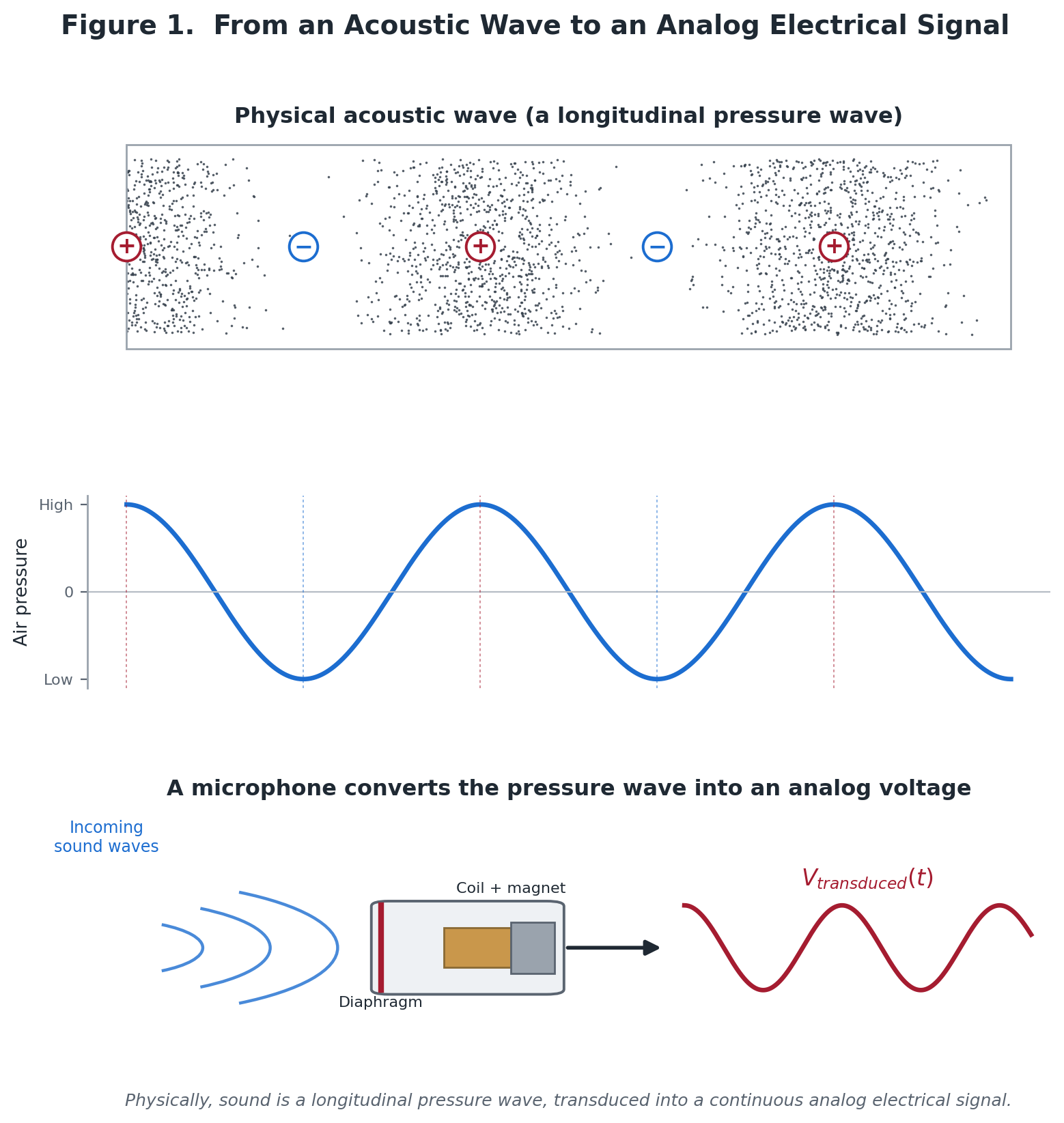
Figure 01: The Mechanical and Electrical Transduction of a Sound Wave. Physically, sound is a longitudinal pressure wave, transduced into a continuous analog electrical signal.
When recording audio, an acoustic transducer such as a microphone diaphragm perceives these pressure waves. The physical displacement of the diaphragm mirrors the continuous fluctuations in air pressure, converting mechanical energy into an analog electrical signal (voltage).
In this analog state, the voltage waveform is an exact mathematical analogy of the acoustic wave. It is perfectly unbroken and continuous: between any two points in time, there exists an infinite number of intermediate voltage values.
3. The Superposition Principle: How Single Data Streams Capture Multi-Faceted Audio
A common conceptual hurdle when first studying digital audio is understanding how a single, linear stream of binary data can capture an entire range of sound like an ensemble of instruments, such as a bass guitar, a human voice, and a treble cymbal, playing simultaneously. This becomes possible as when multiple sound waves occupy the same physical space, they do not travel as isolated vectors. Instead, their pressure variations combine algebraically into a single, highly complex, composite waveform.
The Composite Wave Mechanics
Consider the mathematical behavior of different acoustic registers:
The Bass Register: Low frequencies feature long wavelengths and slow cycles of compression and rarefaction.
The Vocal/Mid Register: Mid-range frequencies feature intermediate wavelengths riding along the broader transitions of the bass waves.
The Treble Register: High frequencies feature rapid, microscopic pressure spikes superimposed onto both the mid-range and bass structures.
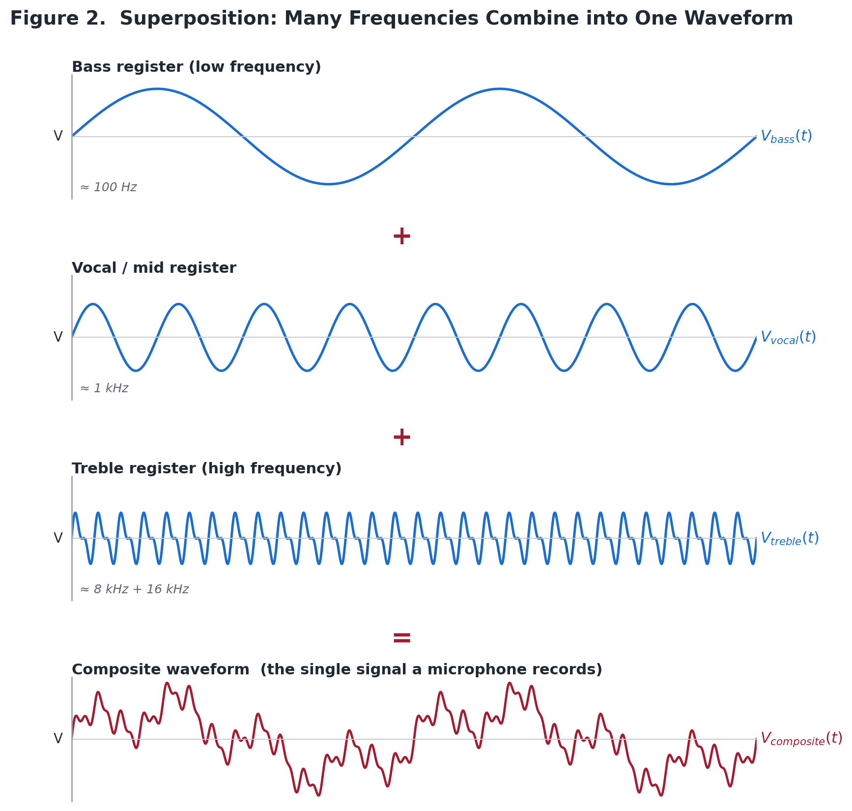
Figure 2: The Superposition Principle and Composite Wave Mechanics - Algebraic Summation of Independent Frequencies into a Single Waveform
When these frequencies converge on a single microphone diaphragm, the microphone registers only one net voltage at any given microsecond. The resulting waveform is jagged and intricate, but it remains a single, continuous function of time.
Pitch as an Emergent Temporal Property
A crucial takeaway for signal processing is that pitch is not an intrinsic property encoded within an isolated audio sample. Instead, pitch is an emergent property determined by the rate of change over time across a series of samples.
By accurately tracing the single, composite line of changing voltages over time, the system inherently captures the macro-bends (low frequencies) and the micro-ripples (high frequencies) simultaneously. When this data is decoded and played back through a speaker, the speaker cone moves in exact accordance with this composite blueprint.
Remarkably, the task of separating the bass, the voice, and the cymbal is left entirely to the ultimate digital signal processor: the human auditory cortex.
4. Converting the Physical World Sound to Digital Audio Data
Step 1: Sampling (Temporal Discretization)
Because a computer cannot store an infinite continuum of values, the analog voltage wave must be sliced into discrete intervals. This temporal slicing is known as sampling. An individual audio sample represents just one value – the amplitude of the sound wave at that discrete point of time. An audio data stream is a sequential, linear array of the samples over time.
In a Mono configuration, each sample contains a single scalar value representing the instantaneous amplitude (voltage height) of the composite wave at that precise microsecond.
In a Stereo configuration, each sample contains a two-element vector representing the synchronous amplitude values for the independent left and right audio channels.
The Nyquist-Shannon Sampling Theorem
The frequency with which these temporal snapshots are taken is defined as the Sampling Rate, measured in Hertz (Hz). To ensure that the discrete digital steps can perfectly reconstruct the original continuous analog wave without losing information, engineers rely on the Nyquist-Shannon Sampling Theorem.
The theorem dictates that to accurately reconstruct a signal, the sampling rate (f_s) must be strictly greater than twice the highest frequency component (f_max) present within the target analog signal:
F_s > 2 ⋅ f_max
The absolute upper limit of healthy human hearing is roughly 20 kHz. Therefore, to capture any pitch audible to humans, an audio system must sample at a rate greater than 40 kHz.
The standard commercial baseline for consumer audio (established by the Red Book CD format) is 44.1 kHz. At this rate, the system records 44,100 individual samples for every single second of audio. This specific frequency provides a safety margin above the 40 kHz threshold, allowing anti-aliasing filters to completely eliminate ultrasonic frequencies that would otherwise cause digital distortion (aliasing).
Step 2: Quantization (Amplitude Discretization)
While sampling discretizes the horizontal axis (time), quantization discretizes the vertical axis (amplitude). Each sample snapshot has a numerical value to represent the magnitude of the wave’s voltage at that instant.
The Resolution Grid and Bit Depth
An analog amplitude value has infinite precision. A digital system, however, must map that value to a fixed numerical scale. This scale is governed by the system’s Bit Depth (n), which dictates the resolution of our digital measurement grid. The total number of available discrete amplitude levels (L) is calculated as:
L = 2^n
| Bit Depth (n) | Available Amplitude Levels (L) | Common Use Case |
|---|---|---|
| 8-bit | 2^8 = 256 | Legacy telecommunications, early computing |
| 16-bit | 2^16 = 65,536 | Standard CD Audio, FLAC, distribution baseline |
| 24-bit | 2^24 = 16,777,216 | Professional studio tracking, mastering archive |
If a system uses an insufficient bit depth (such as 8-bit), the amplitude grid lines are widely spaced. When the actual analog voltage falls between two levels, the system is forced to round the value to the nearest integer. This coarse rounding yields a blocky, stair-stepped approximation of the wave, resulting in severe sonic degradation.
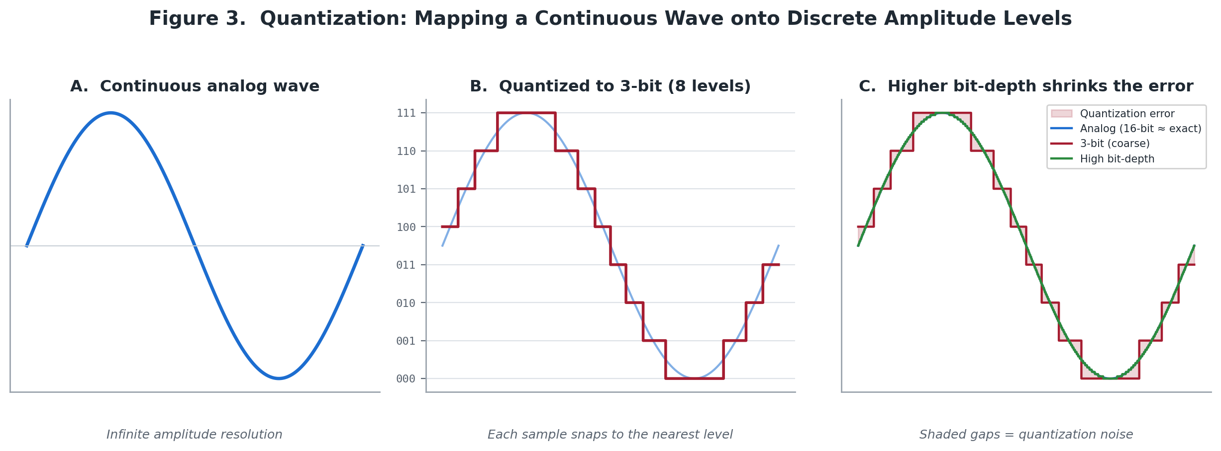
Figure 03: Temporal Discretization and Amplitude Quantization - Comparison of Resolution Grids, Quantization Errors, and Noise Floors.
Quantization Error and the Noise Floor
The mathematical discrepancy introduced by rounding an analog value to a discrete digital level is defined as quantization error. In the audio domain, this error does not present as a distinct digital glitch; rather, it manifests as a stochastic, low-level broadband hiss known as the noise floor.
Every additional bit allocated to the bit depth doubles the vertical resolution, which slashes the quantization error in half. In terms of dynamic range (the ratio between the loudest possible undistorted signal and the quietest perceivable sound), every single bit yields approximately 6 dB of range:
Dynamic Range ≈ 6.02 ⋅ n dB
A 16-bit system provides a dynamic range of roughly 96 dB. This pushes the quantization noise floor well below the threshold of human perception under standard listening conditions.
A 24-bit system expands this range to 144 dB, providing an ultra-low noise floor critical for preventing cumulative noise during multi-track recording and digital signal processing (DSP).
6. Data Packaging: Linear PCM vs. Lossy Compression
Once audio is sampled and quantized, the data must be formatted for storage and transmission.
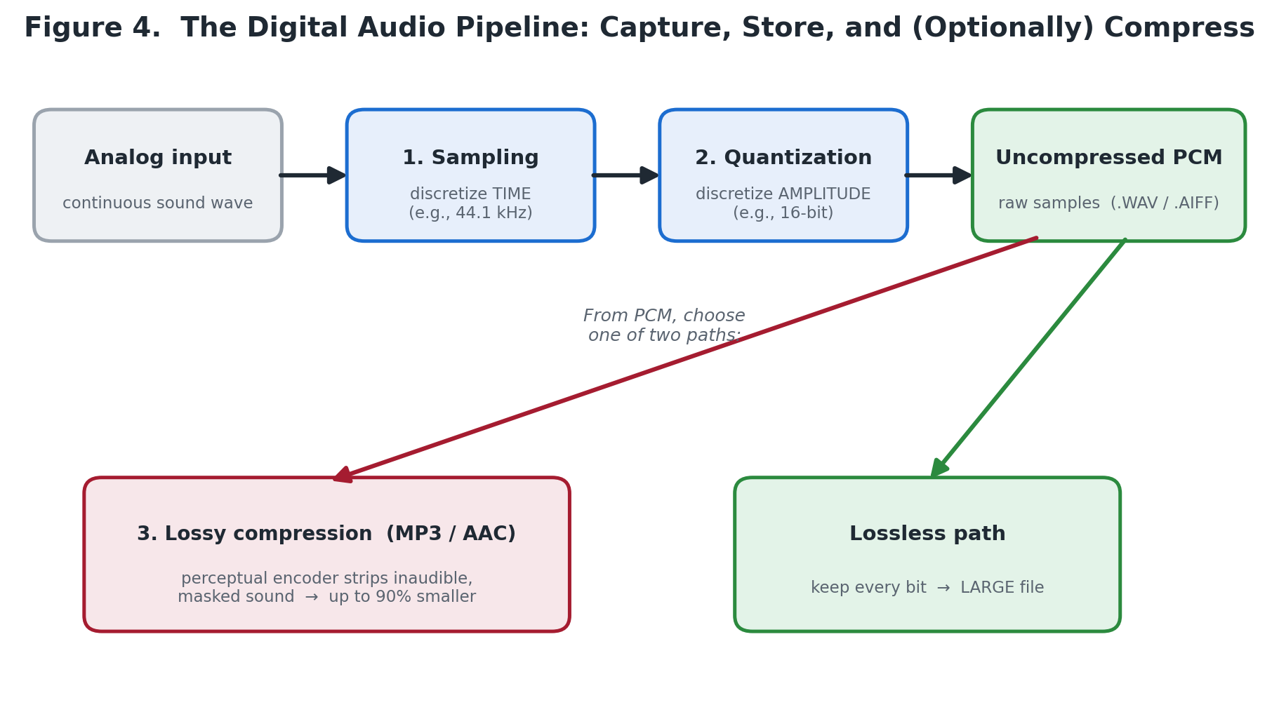
Figure 04: The Digital Audio Conversion and Packaging Pipeline - End-to-End Signal Processing and Storage Architecture
Pulse-Code Modulation (PCM)
The fundamental, uncompressed format for digital audio is Pulse-Code Modulation (PCM). Formats such as .WAV (Microsoft) and .AIFF (Mac) are simply wrapper files containing raw PCM data: a strict, sequential list of binary integers representing the amplitude of each sample.
To calculate the bandwidth or storage footprint of an uncompressed PCM file, we compute the bit rate using the following formula:
Bit Rate = Sampling Rate × Bit Depth × Number of Channels
For a standard CD-quality audio stream (44,100 Hz, 16 bits, 2 channels for stereo):
44,100 × 16 × 2 = 1,411,200 bits per second (bps) ≈ 1,411 kbps
This high data rate demands significant storage architecture—roughly 10.5 MB of data per minute of stereo audio.
Perceptual Coding and Psychoacoustics
To facilitate streaming and network distribution, modern architectures utilize lossy compression formats like MP3 or AAC. Unlike generic data compression algorithms (like .ZIP files), audio compression algorithms exploit the biological limitations of the human auditory system—a discipline known as psychoacoustics.
Lossy encoders analyze the raw PCM stream and apply mathematical models of auditory masking:
Simultaneous Masking: If a high-energy frequency component (e.g., a loud snare drum hit) occurs at the same time as a low-energy, adjacent frequency component (e.g., a quiet synthesizer note), the human ear cannot physically perceive the quieter sound.
Temporal Masking: A loud sound momentarily desensitizes human hearing for a brief window of milliseconds immediately following (and even slightly preceding) the transient spike.
The perceptual encoder identifies these psychoacoustically irrelevant data segments and permanently strips them from the bitstream. By intelligently allocating bits only to sounds the human brain can actively resolve, lossy compression algorithms can reduce file sizes by up to 90% (down to bitrates of 128–320 kbps) while maintaining a high perceived fidelity for the listener.